New experiment

If you installed with “curl” command explained previous chapter, you should have artnew command. This command will make new experiment directory interactively.

Before using this command, please check and make the directory structure!

• rawdata directory (like /mnt/data or /data? Create it to suit your situation.)
• output rootfile directory (like /data/art_output?)
• git repository
  • local repository: suit for online analysis
  • remote repository: suit for offline analysis

Let’s start “artnew” command!

The word after “:” is your input.

> artnew

1. Input the experiment name

create new artemis work directory? (y/n): y
Input experimental name: test
Is it OK? (y/n): y
Input value: test

2. Check the base directory (default value is fine!) If there are no input, the default value will be used.

artnew: If no input is provided, the default value is used.
Input repository path or URL (default: https://github.com/okawak/artemis_crib.git):
Is it OK? (y/n): y
Input value: https://github.com/okawak/artemis_crib.git

3. Input the rawdata directory

Input rawdata directory path (default: /data/test/ridf):
Is it OK? (y/n): y
Input value: /data/test/ridf

4. Input the output directory

Input output data directory path (default: /data/test/user):
Is it OK? (y/n): y
Input value: /data/test/user

5. Input the git setting (PLEASE MAKE your own repository. Local repository will be fine)

Based on the repository, do you make your own repository? (y/n): y
is it local repository (y/n): y
artnew: making LOCAL repository of test
Input the local repository path (default: $HOME/repos/exp):
Is it OK? (y/n): y
Input value: /home/crib/repos/exp

-- snip --

art_analysis setting for test is finished!

The initial setting is completed!!

New user

After artnew command, you can see new directory of config files.

 > tree -a art_analysis
 art_analysis
 ├── .conf
 │   ├── artlogin.sh
+│   └── test.sh
 ├── bin
 │   ├── art_check
 │   ├── art_setting
 │   └── artnew
+└── test

This is experiment name “test” example. In order to load this script test.sh, please modify “EXP_NAME” environment valiable in .zshrc.

export EXP_NAME="test" # your experiment

And load the config file.

> source ~/.zshrc

Then you can make your own work directory by using artlogin command!

Let’s start “artlogin” command!

For example, let’s make default user (user name is the same with experiment name)!

> artlogin

If you want to make your own directory, the following will work.

> artlogin yourname

1. Check if you really want to make your work directory

artlogin: user 'test' not found.
create new user? (y/n): y
Cloning into '/Users/okawa/art_analysis/test/test'...
done.

2. Git setting

artlogin: making local git config
Input fullname: KodaiOkawa
Is it Okay? (y/n): y
Input email address: okawa@cns.s.u-tokyo.ac.jp
Is it Okay? (y/n): y

3. Symbolic link setting. If there are no problem, the current directory move to your artemis work directory

> pwd
/home/crib/art_analysis/test/test
> ls -l

If your synbolic link seems okay, the setting is all!

If artnew setting have problem, the error message will appear. Typical examples are as follows.

mkdir: /data: Read-only file system

This is a case of the directory permissions not being set correctly. Use the chmod command or similar to set them correctly and try again.

Build

Before starting analysis, you need to build. The current version of the artemis use “cmake” so the following steps must be taken.

> artlogin (username)
> mkdir build && cd build
> cmake ..
> make -j4
> make install
> acd

acd is the alias command that is definded after artlogin command. (acd = cd your_work_directory) Also if you changed some processor, you need to do these process.

Then some important configuration files are automatically created.

 > tree -L 1
 .
+├── artemislogon.C
+├── thisartemis-crib.sh

 -- snip --

 └── run_artemis.cpp

Before starting artemis, you need to load the thisartemis-crib.sh. The artlogin command is also used to read this script, so run this command again after the build.

> artlogin (usename)
> a

Then you can start artemis by using a command!

artemis commands

Before configuring the settings according to your experiment, let’s check that artemis is working!

> artlogin (username)
> a # start the artemis!

Then the prompt change to the artemis [0]. This means you are in artemis console!

Analysis using artemis use event loop. It is therefore necessary to load a file that specifies what kind of analysis is to be performed. This file is called the steering file. As an example, let’s check the operation using a steering file that only generates random numbers!

The command to load the steering file is add.

artemis [0] add steering/example/example.tmpl.yaml NUM=0001 MAX=10

This means that 10000 random numbers from 0 to MAX=10 are generated (10000 event loops). NUM=0001 is the ID, so any number is okay (related to outputed file name).

And the command to start the event loop is resume. (Often abbreviated as “resume” or “re”. The abbreviated form will also run without problems if there are no conflicts with other commands.)

artemis [1] res
artemis [2] Info in <art::TTimerProcessor::PostLoop>: real = 0.02, cpu = 0.02 sec, total 10000 events, rate 500000.00 evts/sec

When the time taken for such an analysis is displayed, it means that all event loops have been completed. If you are doing a time-consuming analysis and want to suspend the event loop in the middle, suspend command is used. (Often “sus” or “su” is used.)

artemis [2] sus

This event loop creates histogram objects (inherit from TH1 or TH2) and a TTree object. Let’s look at how to access each of these.

Histogram

Details are given in the Histograms section, but histograms are created in an internal directory. To access it, you need to use the same commands as for the linux command, such as “ls” or “cd”, to get to that directory.

artemis [2] ls

 artemis
>   0 art::TTreeProjGroup test2           test (2) # the first ">" means your current position
    1 art::TTreeProjGroup test            test
    2 art::TAnalysisInfo analysisInfo

# then let's move to the "test" directory!

artemis [3] cd 1
artemis [4] ls

 test
>   0 art::TH1FTreeProj hRndm           random value

You can use the command ht [ID] to display a histogram. The ID can be omitted if it is already represented by >.

artemis [5] zone # make artemis canvas
artemis [6] ht 0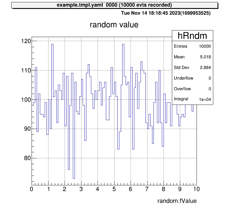

Next, let’s also check the histogram in “test2” directory and display two histograms vertically at the same time!

artemis [7] zone 2 1 # row=2, column=1
artemis [8] ht 0 # show the current hist 
artemis [9] cd ..
artemis [10] ls

 artemis
>   0 art::TTreeProjGroup test2           test (2)
    1 art::TTreeProjGroup test            test
    2 art::TAnalysisInfo analysisInfo

artemis [11] cd 0

 test2
>   0 art::TH1FTreeProj hRndm2          random number

artemis [12] ht 0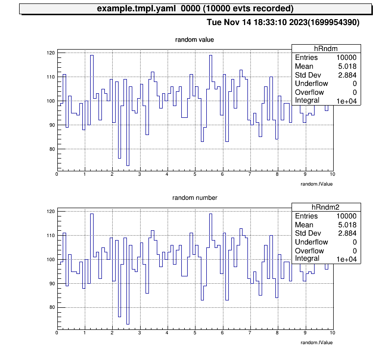

TTree

Now consider displaying a diagram from a TTree object. The file is created at here.

artemis [13] fls
 files
    0 TFile output/0001/example_0001.tree.root            (CREATE)

We use the fcd command to navigate to this root file.

artemis [14] fcd 0
artemis [15] ls

 output/0001/example_0001.tree.root
>   0 art::TAnalysisInfo analysisInfo
    1 art::TArtTree tree            tree

The command branchinfo (“br”) displays a list of the branches stored in this tree.

artemis [16] br
random               art::TSimpleData

At the same time, the ROOT command can be used.

artemis [17] tree->Print()
******************************************************************************
*Tree    :tree      : tree                                                   *
*Entries :    10000 : Total =          600989 bytes  File  Size =      86144 *
*        :          : Tree compression factor =   7.00                       *
******************************************************************************
*Br    0 :random    : art::TSimpleData                                       *
*Entries :    10000 : Total  Size=     600582 bytes  File Size  =      85732 *
*Baskets :        1 : Basket Size=    3200000 bytes  Compression=   7.00     *
*............................................................................*

Accessing data in a branch’s data class requires the use of public variables and methods, which can be examined by providing arguments to branchinfo [branch name] or classinfo [class name].

artemis [18] br random

 art::TSimpleData

 Data Members


 Methods

                   Bool_t   CheckTObjectHashConsistency
             TSimpleData&   operator=
             TSimpleData&   operator=

 See also

     art::TSimpleDataBase<double>

artemis [19] cl art::TSimpleDataBase<double>

 art::TSimpleDataBase<double>

 Data Members

                   double   fValue

 Methods

                     void   SetValue
                   double   GetValue
                   Bool_t   CheckTObjectHashConsistency
     TSimpleDataBase<double>&   operator=

 See also

     art::TDataObject       base class for data object

Therefore, it can be seen that it can be accessed by the value fValue.

artemis [20] zone
artemis [21] tree->Draw("random.fValue>>(100,0.,10.)")

Other useful commands

artemis [*] help # show the commands we can use
artemis [*] save # save the current canvas
artemis [*] print # print the current canvas (send to the printer, need to configure)
artemis [*] unzoom
artemis [*] lgy, lgz, lny, lnz # linear or log scale

Map configuration

From this section, we start to configure the settings according to the actual experimental setup. The setting files are followings:

> tree
.
├── mapper.conf
├── conf
│   ├── map
│   │   ├── ppac
│   │   │   ├── dlppac.map

-- snip --

│   └── seg
│       ├── modulelist.yaml
│       └── seglist.yaml

-- snip --

1. What is the map file?

The data obtained from an ADC/TDC is in the form of, for example, “The data coming into channel 10 of an ADC with an ID of 1 is 100”.

---
title: Data flow example
---
graph LR;
    A{detector} -->|signal| B(TDC/ADC<br></br>ID=1, ch=10)
    B -->|value=100| C[<strong>Data build</strong>\nridf file]

The role of the map file is to map this value of “100” to an ID that is easy to analyse. An ID that is easy to analyse means, for example, that even if signals from the same detector are acquired with different ADCs/TDCs, the same ID is easier to handle in the analysis.

---
title: Data flow example
---
graph LR;
    A(TDC/ADC<br></br>ID=1, ch=10) -->|value=100| B[<strong>Data build</strong>\nridf file]
    B -->|value=100 mapping to| C(analysis<br></br>ID=2, ch=20)

After mapping, we can check the data of this “100” from ID=2 and ch=20. This ID and channel (2, 20) are provided for convenience, so you can freely set them.

So, in summary, the map file role is like this:

---
title: role of the map file
---
graph LR;
    A(DAQ ID<br></br>ID=1, ch=10) <-->|mapping| B(analysis ID<br></br>ID=2, ch=20)

2. map files

CRIB is using Babirl for the DAQ system. In this system, the DAQ ID represented in the example is determined by five parameters.

• device ID (dev)
• focal plane (fp)
• detector ID (det)
• geometry ID (geo)
• channel (ch)

The dev, fp, det and geo parameters can be set from DAQ setting. For the CRIB experiment, conventionally we set dev=12, fp=0–2 (for each MPV), det=6,7 (6=energy, 7=timing) and geo=from 0. But you can change it freely.

And analysis ID represented in the example is determined by two parameters.

• Category ID (CatID, cid)
• id (fID)

Of cource you can also set the value freely.

The format of the map file is followings:

# [category] [id] [[device] [focus] [detector] [geo] [ch]] ....
   1,   0,  12,   1,  6,   0,   0

# map for SSD
# [category] [id] [[device] [focus] [detector] [geo] [ch]] ....
#
# Map: energy, timing
#
#--------------------------------------------------------------------
   1,   0,  12,   1,  6,   0,   0,  12,   2,  7,   0,   0

Please create map files for all detectors like this!

3. mapper.conf

You can select the map file to be loaded with this file. This is especially useful when separating map files for testing from map files for the experiment.

The format is followings: (path/to/the/map/file number)

# file path for configuration, relative to the working directory
# (path to the map file) (Number of columns)

# cid = 1: rf
conf/map/rf/rf.map 1

In the note example above, the number is 2.

Please do not forget to add to the mapper.conf after you add some map files.

4. (option) segment files

This conf files are used when you use “chkseg.yaml” steering file. This steering file create raw data 2D histograms. I will describe in the Example: online_analysis/Check raw data in detail.

Steering

The steering file (yaml format) is a file that directs the process of how the obtained data is to be processed. The artemis is an object-oriented program whose components are called processors, which are combined to process data.

The main role of the “processor” is to process data from an input data called InputCollection and create an output data called OutputCollection. This “OutputCollection” will be stored into the root file as a “tree”. Complex processing can be performed by using “processor” in multiple steps.

I will explain how to create this “steering” file using Si detector data as an example.

---
title: example of the data process structure
---
graph TD;
    subgraph event loop
    A-->B(mapping processor<br></br>InputCollection: decoded data\nOutputCollection: Si raw data)
    B-->C(calibration processor<br></br>InputCollection: Si raw data\nOutputCollection: Si calibrated data)
    C-->X((event end))
    X-->A
    end
    subgraph DAQ
    D(Raw binary data)-->A(decode processor<br></br>InputCollection: raw data\nOutputCollection: decoded data)
    end

Steering file: Silicon data case

First, I describe what is the Anchor and how to use command line arguments. See example here.

Anchor:
 - &input ridf/@NAME@@NUM@.ridf
 - &output output/@NAME@/@NUM@/chkssd@NAME@@NUM@.root
 - &histout output/@NAME@/@NUM@/chkssd@NAME@@NUM@.hist.root

You can use variables from elsewhere in the steering file by declaring them as such. For example if you write:

something: *input

This unfolds as follows:

something: ridf/@NAME@@NUM@.ridf

Variables enclosed in @ can also be specified by command line arguments. For example, If you command like the following in the artemis console,

artemis [1] add steering/chkssd.yaml NAME=run NUM=0000

it is considered as

Anchor:
 - &input ridf/run0000.ridf
 - &output output/run/0000/chkssdrun0000.root
 - &histout output/run/0000/chkssdrun0000.hist.root

1. General processor

When using the “Babirl”, the data file will be in the form of “ridf”. In this case, the beginning and end of the steering file is usually as follows.

Processor:
  - name: timer
    type: art::TTimerProcessor

  - name: ridf
    type: art::TRIDFEventStore
    parameter:
      OutputTransparency: 1
      InputFiles:
        - *input
      SHMID: 0

  - name: mapper
    type: art::TMappingProcessor
    parameter:
      OutputTransparency: 1

# -- snip --

  - name: outputtree
    type: art::TOutputTreeProcessor
    parameter:
      FileName:
        - *output

• TTimerProcessor: measure the time taken to process data
• TRIDFEventStore: decode the ridf file and store the value in EventStore (see below)
• TMappingProcessor: read mapper.conf for mapping
• TOutputTreeProcessor: writes data to the root file

OutputTransparency is set to 1, indicating that “OutputCollection” is not exported to the root file.

2. Mapping processor

The “mapping processor” puts the data stored in the “EventStore” into a certain data class based on “mapper.conf”. Assume the following map file is used.

# map for SSD
# [category] [id] [[device] [focus] [detector] [geo] [ch]] ....
#
# Map: energy, timing
#
#--------------------------------------------------------------------
   1,   0,  12,   1,  6,   0,   0,  12,   2,  7,   0,   0

In this case, since we are assuming data from the Si detector, let’s consider putting it in a data class that stores energy and timing data, “TTimingChargeData”! The processor mapping to this data class is “TTimingChargeMappingProcessor”.

Processor:
  - name: proc_ssd_raw
    type: art::TTimingChargeMappingProcessor
    parameter:
      CatID:         1
      ChargeType:    1
      ChargeTypeID:  0
      TimingTypeID:  1
      Sparse:        1
      OutputCollection: ssd_raw

1. CatID: enter here the same number as the cid (category ID) in the map file.
2. ChargeType: there are various ways to store energy (charge) and timing using this processor, but this time “1” is specified to use the processing method using ADC and TDC.
3. Charge/TimingTypeID: The map file has two sets of five parameters that specify the DAQ ID. Which of these parameters specifies which represents the energy (charge) and timing. (it start from “0”)
4. Sparse: parameter for the output data structure
5. OutputCollection: name of the data class to be output

Then, you can access the ssd_raw data by using like tree->Draw("ssd_raw.fCharge")

3. Calibration processor

While the data in the “ssd_raw” are raw channel of the ADC and TDC, it is important to see the data calibrated to energy and time. I will explain the details in Example: preparation/macro, but here I will discuss the calibration processors assuming that the following appropriate calibration files have been created.

• prm/ssd/ch2MeV.dat
• prm/ssd/ch2ns.dat

Now, let’s load these files.

Processor:
  - name: proc_ssd_ch2MeV
    type: art::TParameterArrayLoader
    parameter:
      Name: prm_ssd_ch2MeV
      Type: art::TAffineConverter
      FileName: prm/ssd/ch2MeV.dat
      OutputTransparency: 1

  - name: proc_ssd_ch2ns
    type: art::TParameterArrayLoader
    parameter:
      Name: prm_ssd_ch2ns
      Type: art::TAffineConverter
      FileName: prm/ssd/ch2ns.dat
      OutputTransparency: 1

To calibrate data contained in a TTimingChargeData class, a TTimingChargeCalibrationProcessor processor is used.

Processor:
  - name: proc_ssd
    type: art::TTimingChargeCalibrationProcessor
    parameter:
      InputCollection:      ssd_raw
      OutputCollection:     ssd_cal
      ChargeConverterArray: prm_ssd_ch2MeV
      TimingConverterArray: prm_ssd_ch2ns

Note here that “InputCollection”, “ChargeConverterArray”, and “TimingConverterArray” use the same names as the highlighted lines in the code block above.

> artlogin (username)
> a
artemis [0] processordescription art::TTimingChargeCalibrationProcessor
Processor:
  - name: MyTTimingChargeCalibrationProcessor
    type: art::TTimingChargeCalibrationProcessor
    parameter:
      ChargeConverterArray: no_conversion  # [TString] normally output of TAffineConverterArrayGenerator
      InputCollection: plastic_raw  # [TString] array of objects inheriting from art::ITiming and/or art::ICharge
      InputIsDigital: 1  # [Bool_t] whether input is digital or not
      OutputCollection: plastic  # [TString] output class will be the same as input
      OutputTransparency: 0  # [Bool_t] Output is persistent if false (default)
      TimingConverterArray: no_conversion  # [TString] normally output of TAffineConverterArrayGenerator
      Verbose: 1  # [Int_t] verbose level (default 1 : non quiet)

4. Split files

If you want to analyse a large number of detectors, not just Si detectors, writing everything in one steering file will result in a large amount of content that is difficult to read.

In that case, we can use “include” node!

In the examples we have written so far, let’s only use a separate file for the part related to the analysis of the Si detector.

# -- snip --

Processor:

# -- snip --

  - include: ssd/ssd_single.yaml

# -- snip --

Processor:
# parameter files
  - name: proc_ssd_ch2MeV
    type: art::TParameterArrayLoader
    parameter:
      Name: prm_ssd_ch2MeV
      Type: art::TAffineConverter
      FileName: prm/ssd/ch2MeV.dat
      OutputTransparency: 1

  - name: proc_ssd_ch2ns
    type: art::TParameterArrayLoader
    parameter:
      Name: prm_ssd_ch2ns
      Type: art::TAffineConverter
      FileName: prm/ssd/ch2ns.dat
      OutputTransparency: 1

# data process
  - name: proc_ssd_raw
    type: art::TTimingChargeMappingProcessor
    parameter:
      CatID:         1
      ChargeType:    1
      ChargeTypeID:  0
      TimingTypeID:  1
      Sparse:        1
      OutputCollection: ssd_raw

  - name: proc_ssd
    type: art::TTimingChargeCalibrationProcessor
    parameter:
      InputCollection:      ssd_raw
      OutputCollection:     ssd_cal
      ChargeConverterArray: prm_ssd_ch2MeV
      TimingConverterArray: prm_ssd_ch2ns

In this way, the contents of “chkssd.yaml” can be kept concise, while the same process is carried out. Note that the file paths here are relative to the paths from the steering directory. Parameter files, for example, are relative paths from the working directory (one level down).

Utilising file splitting also makes it easier to check the steering files that analyse a large number of detectors like this.

# -- snip --

Processor:

# -- snip --

  - include: rf/rf.yaml
  - include: ppac/f1ppac.yaml
  - include: ppac/dlppac.yaml
  - include: mwdc/mwdc.yaml
  - include: ssd/ssd_all.yaml

# -- snip --

Summary

The whole steering file is as follows:

Anchor:
 - &input ridf/@NAME@@NUM@.ridf
 - &output output/@NAME@/@NUM@/chkssd@NAME@@NUM@.root
 - &histout output/@NAME@/@NUM@/chkssd@NAME@@NUM@.hist.root

Processor:
  - name: timer
    type: art::TTimerProcessor

  - name: ridf
    type: art::TRIDFEventStore
    parameter:
      OutputTransparency: 1
      InputFiles:
        - *input
      SHMID: 0

  - name: mapper
    type: art::TMappingProcessor
    parameter:
      OutputTransparency: 1

  - include: ssd/ssd_single.yaml

# output root file
  - name: outputtree
    type: art::TOutputTreeProcessor
    parameter:
      FileName:
        - *output

Processor:
# parameter files
  - name: proc_ssd_ch2MeV
    type: art::TParameterArrayLoader
    parameter:
      Name: prm_ssd_ch2MeV
      Type: art::TAffineConverter
      FileName: prm/ssd/ch2MeV.dat
      OutputTransparency: 1

  - name: proc_ssd_ch2ns
    type: art::TParameterArrayLoader
    parameter:
      Name: prm_ssd_ch2ns
      Type: art::TAffineConverter
      FileName: prm/ssd/ch2ns.dat
      OutputTransparency: 1

# data process
  - name: proc_ssd_raw
    type: art::TTimingChargeMappingProcessor
    parameter:
      CatID:         1
      ChargeType:    1
      ChargeTypeID:  0
      TimingTypeID:  1
      Sparse:        1
      OutputCollection: ssd_raw

  - name: proc_ssd
    type: art::TTimingChargeCalibrationProcessor
    parameter:
      InputCollection:      ssd_raw
      OutputCollection:     ssd_cal
      ChargeConverterArray: prm_ssd_ch2MeV
      TimingConverterArray: prm_ssd_ch2ns

> acd
> a
artemis [0] add steering/chkssd.yaml NAME=run NUM=0000

Histograms

In the online analysis, it is important to have immediate access to data. The artemis can produce TTree object but long commands are needed to access, for example,

artemis [1] fcd 0  # move to the created rootfile
artemis [2] zone 2 2  # make a "artemis" 2x2 canvas
artemis [3] tree->Draw("ssd_cal.fCharge:ssd_cal.fTiming>(100,0.,100., 100,0.,100)","ssd_cal.fCharge > 1.0","colz")

This would take time if there are some histograms that you want to display immediately…

Therefore, if you know in advance the diagram you want to see, it is useful to predefine its histogram! The processor used is TTreeProjectionProcessor. I would like to explain how to use this one.

1. Steering file

Let’s look at how histograms are defined when looking at SSD data. First, let’s prepare the steering file as follows! please see previous section for omissions.

# -- snip --

  - include: ssd/ssd_single.yaml

# Histogram
  - name: projection_ssd
    type: art::TTreeProjectionProcessor
    parameter:
      FileName: hist/ssd/ssd.yaml
      Type:     art::TTreeProjection
      OutputFilename: *histout


# output root file
  - name: outputtree
    type: art::TOutputTreeProcessor
    parameter:
      FileName:
        - *output

The histogram is created based on the TTree object, so describe the processing of the histogram after the part that represents the data processing and before the part that outputs the TTree (TOutputTreeProcessor).

There are three points to note here.

1. It is possible to create a root file containing only a histogram as well as a root file containing a TTree. (Look at the node part of the OutputFilename.)
2. The histogram itself is defined in a separate file to this one, written on the highlighted line above.
3. The file paths are relative to the working directory.

Therefore, I would now like to show the histogram definition file.

2. Histogram file

First please look at this example.

 1anchor: 
 2  - &energy ["ssd_cal.fCharge",100,0.,100.]
 3  - &timing ["ssd_cal.fTiming",100,0.,100.]
 4alias:
 5  energy_cut: ssd_cal.fCharge>1.0;
 6group:
 7  - name: ssd_test
 8    title: ssd_test
 9    contents:
10      - name: ssd_energy
11        title: ssd_energy
12        x: *energy
13
14      - name: ssd_timing
15        title: ssd_timing
16        x: *timing
17
18      - name: ssd_energy and timing
19        title: ssd_energy and timing
20        x: *timing
21        y: *energy
22        cut: energy_cut

This definition file consists of three parts.

2.1 anchor

The actual core part is the “2.3 group”, but “2.1 anchor” and “2.2 alias” are often used to make this part easier to write. The anchor defines the first argument of tree->Draw("ssd_cal.fCharge>(100,0.,100.)","ssd_cal.fCharge > 1.0")

The array stored in the variable named “energy” in the second line looks like [str, int, float, float] and has the following meanings

1. str: Name of the object (need double quote “”)
2. int: Number of bins of histogram
3. float: Minimum value of histogram range
4. float: Maximum value of histogram range

As you might imagine, inside the first argument you can also add operations such as TMath::Sqrt(ssd_cal.fCharge) or ssd_cal.fCharge-ssd_cal.fTiming, because it is the same with “tree->Draw”.

Note, however, that the definition here is for one-dimensional histograms. Two-dimensional histograms will be presented in Section 2.3. It is very simple to write!

2.2 alias

This part is used when applying gates to events (often we call it as “cut” or “selection”). For example, if you only want to see events with energies above 1.0 MeV, you would write something like tree->Draw("energy","energy>1.0").

The alias node is used to define the part of energy>1.0

2.3 group

The histogram is defined here and the object is stored in a directory in artemis (ROOT, TDirectory). In the example shown above, the directory structure would look like this:

(It is not actually displayed in this way).

# in artemis
.
└── ssd_test
    ├── ssd_energy (1D hist)
    ├── ssd_timing (1D hist)
    └── ssd_energy and timing (2D hist)

The first “name” and “title” nodes are arguments of TDirectory instance. Also the second “name” and “title” nodes are arguments of instance of TH1 or TH2 object. The other “x”, “y” and “cut” is the important node!

1. If there are only “x” nodes -> 1D histogram
2. If there are both “x” and “y” nodes -> 2D histogram
3. In any case, it can be gated by adding a “cut” node.

3. Commands for histograms

There are many useful command for checking the histogram objects. These are similar to the ANAPAW commands.

1. ls : check the artemis directory

> artlogin (username)
> a

artemis [0] add steering/chkssd.yaml NAME=hoge NUM=0000
artemis [1] res
artemis [2] sus
artemis [3] ls # check the artemis directory

 artemis
>   0 art::TTreeProjGroup ssd_test        ssd_test
    1 art::TAnalysisInfo analysisInfo

2. cd [ID] : move to the directory of the ID

artemis [4] cd 0
artemis [5] ls

 ssd_test
>   0 art::TH1FTreeProj ssd_energy      ssd_energy
    1 art::TH1FTreeProj ssd_timing      ssd_timing
    2 art::TH2FTreeProj ssd_energy and timing ssd_energy and timing

3. ht [ID] [option] : draw the histogram of the ID

artemis [6] ht 0
artemis [7] ht 2 colz

4. hn : draw the next ID histogram
5. hb : draw the prev ID histogram

4. Template hist file

When setting up several detectors of the same type and wanting to set up a histogram with the same content, it is tedious to create several files with only the names of the objects changed. In such cases, it is useful to allow the histogram definition file to have arguments.

Please look here first.

# -- snip --

  - include: ssd/ssd_single.yaml

# Histogram
  - name: projection_ssd
    type: art::TTreeProjectionProcessor
    parameter:
      FileName: hist/ssd/ssd.yaml
      Type:     art::TTreeProjection
      OutputFilename: *histout
      Replace: |
        name: ssd_cal        

# -- snip --

We add the highlighted lines. Then the “name” can be used at hist file by @name@! The “name” can be freely set.

anchor: 
  - &energy ["@name@.fCharge",100,0.,100.]
  - &timing ["@name@.fTiming",100,0.,100.]
alias:
  energy_cut: @name@.fCharge>1.0;
group:
  - name: ssd_test
    title: ssd_test
    contents:
      - name: ssd_energy
        title: ssd_energy
        x: *energy

      - name: ssd_timing
        title: ssd_timing
        x: *timing

      - name: ssd_energy and timing
        title: ssd_energy and timing
        x: *timing
        y: *energy
        cut: energy_cut

This is useful when there are more objects to check!

# -- snip --

  - include: ssd/ssd_single.yaml

# Histogram
  - name: projection_ssd
    type: art::TTreeProjectionProcessor
    parameter:
      FileName: hist/ssd/ssd.yaml
      Type:     art::TTreeProjection
      OutputFilename: *histout
      Replace: |
        name: ssd_cal        

  - name: projection_ssd
    type: art::TTreeProjectionProcessor
    parameter:
      FileName: hist/ssd/ssd.yaml
      Type:     art::TTreeProjection
      Replace: |
        name: ssd_raw        
  # and so on!

# -- snip --

File splitting using “include” nodes, as described in the section on steeling, can also be used in the same way.

VNC server

When we start the analysis, there are many situations where the analysis server on which artemis is installed is not only operated directly, but also remotely using “ssh”. In such cases, there are various settings that need to be made in order for the figure to be displayed on the local computer, and some of these methods are described in this section. We recommended to use VNC server currently, but note that policies may change in the future.

This is a list of ways to display the figures.

• X11Forwarding
• VNC server
• Save figure and check by using VScode
• Web browser (THttpServer)

X11Forwarding

This is the simplest method. Simply transfer the remote X to the local.

ssh -X analysisPC

This “X” option allow the X11Forwarding.

However, the problem with this method is that it takes a long time to process, and it takes longer from the time the command is typed until it is drawn. It is also not recommended as the process can become slow if a large number of people use it at the same time.

However, it is simpler than other methods and should be used when necessary, e.g. for debugging.

VNC server

First please install VNC viewer to your PC. Any viewer may work well, but we are using this software.

First, please check the ID number of the VNC server we are running.

> vncserver -list

TigerVNC server sessions:

X DISPLAY #	PROCESS ID
:1		  3146
:5		  7561
:2022	  29499
:2		  23055

In this example, number 1, 5, 2022 and 2 VNC server is running. And select an available number to start the VNC server you want to use.

> vncserver :10 # start the VNC server!

If you want to kill the VNC server, the below command will work.

> vncserver -kill :10 # kill the VNC server!

Next, configure the canvas created by artemis to be sent to a VNC server. The a command can treat this process by using .vncdisplay file!

> artlogin (username) # move to your artemis work directory
> echo "10" > .vncdisplay # write the ID of VNC server to the .vncdisplay file

Then, the setting in analysis PC is completed! The next step is to set up your local PC to receive this.

In this section, we are assuming that you have a CNS login server account.

To access the analysis PC, use two-stage ssh. Prepare the following configuration file.

Host login
    # need to change
    HostName CNS_loginserver_hostname
    User username
    IdentityFile ~/.ssh/id_rsa
    # no need to change (if you want)
    ForWardX11Timeout 24h
    ControlPersist 30m
    ForwardAgent yes
    ControlMaster auto
    ControlPath ~/.ssh/mux-%r@%h:%p

# any name is okay
Host analysis
    # need to change
    HostName analysisPC_hostname
    User username
    IdentityFile ~/.ssh/id_rsa
    # no need to change (if you want)
    ProxyCommand ssh login nc %h %p
    ForwardAgent yes
    ControlMaster auto
    ControlPath ~/.ssh/mux-%r@%h:%p
    ControlPersist 30m

Then you can access to the analysis PC simply by:

> ssh analysis

Next, in order to receive from the VNC server, we use port-forwarding! VNC servers with ID x use port number 5900+x. For example if we use number “10”, the port will be 5910.

Forward this to a certain port on localhost. This number can be any number that is not in use.

---
title: An example of port-forwarding
---
graph LR;
    A(analysis PC<br></br>port 5910) --> |send|B(local PC<br></br>port 55910)

Host analysis
    HostName analysisPC_hostname
    User username
    IdentityFile ~/.ssh/id_rsa
    LocalForward 55910 localhost:5910
    ProxyCommand ssh login nc %h %p
    ForwardAgent yes
    ControlMaster auto
    ControlPath ~/.ssh/mux-%r@%h:%p
    ControlPersist 30m

This allows you to display a VNC display by accessing port 55910 on your own PC (localhost), instead of having to access port 5910 on the analysis PC!

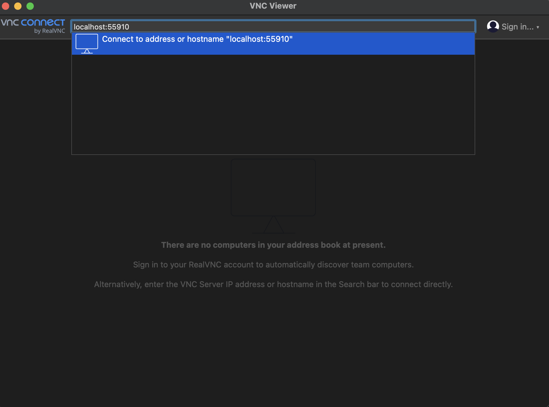
If your PC is in the same network, changing “localhost” to the “IP address of analysis PC” is okay (ex. 192.168.1.10:5910).

Save figure and check by using VScode

VScode is very exciting editor! The extension supports ssh and allows remote png files to be displayed on the editor.

However, it is a bit time-consuming as the diagram has to be saved each time to view it. Please refer to this as one method.

Web browser (THttpServer)

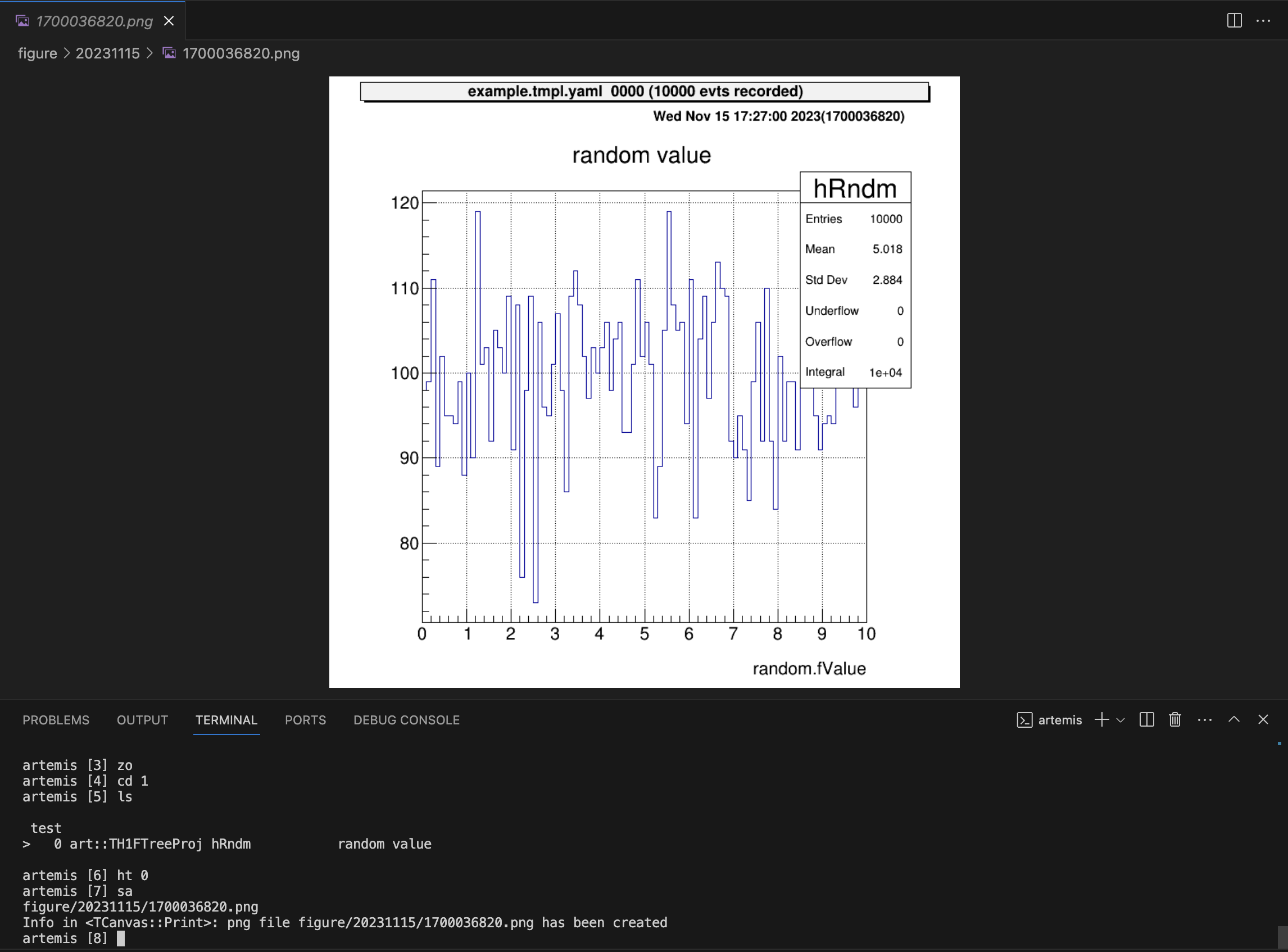
This is option…

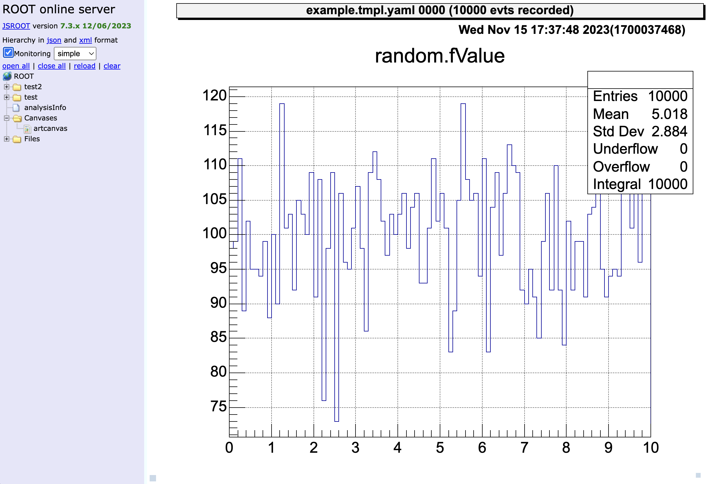
Now the histogram object cannot display by JSROOT, because the object is not actually “TH1” or “TH2” object but “TH1FTreeProj” or “TH2FTreeProj”. (ref: issue#40)

We can only display the “TCanvas” Object.