Chapter 1
Installation
This chapter describes how to set up the artemis environment for the CRIB experiment.
This chapter describes how to set up the artemis environment for the CRIB experiment.
The following machines have been tested for operation.
sudo apt-get install binutils cmake dpkg-dev g++ gcc \
libssl-dev git libx11-dev \
libxext-dev libxft-dev libxpm-dev python3 libtbb-dev \
libvdt-dev libgif-dev \
gfortran libpcre3-dev \
libglu1-mesa-dev libglew-dev libftgl-dev \
libfftw3-dev libcfitsio-dev libgraphviz-dev \
libavahi-compat-libdnssd-dev libldap2-dev \
python3-dev python3-numpy libxml2-dev libkrb5-dev \
libgsl-dev qtwebengine5-dev nlohmann-json3-dev libmysqlclient-dev \
libyaml-cpp-dev
NOTE:
Artemis uses ROOT library. For detailded information, please refer Installing ROOT
This is one example to install the ROOT from the source.
# You may update your local copy by issuing a `git pull` command from within `root_src/`.
cd install_dir
git clone https://github.com/root-project/root.git root_src
# check out the tag to specify the ROOT version
cd root_src
git checkout -b v6-30-04 refs/tags/v6-30-04
cd ..

mkdir root_build root_install && cd root_build
cmake -DCMAKE_INSTALL_PREFIX=../root_install -Dmathmore=ON ../root_src # && check cmake configuration output for warnings or errors
make -j4
make install
source ../root_install/bin/thisroot.sh # or thisroot.{fish,csh}
If there are any problems at the compile, additional packages may need to be installed. See also dependencies.
I recommend to write source thisroot.sh part in the .bashrc/.zshrc to load this library.
From the current situation, CRIB experiment doesn’t use GET system, so we describe how to install it without linking it to GET decoder.
Also, it can link to openMPI, but the below commands assume not using openMPI.
See artemis repo for more information.
cd hoge
git clone https://github.com/artemis-dev/artemis.git -b develop
cd artemis
mkdir build
cd build
cmake -DCMAKE_INSTALL_PREFIX=../install ..
make -j4
make install
source ../install/bin/thisartemis.sh
Then, <CMAKE_INSTALL_PREFIX>/bin/thisartemis.sh will be created
and this shell script can configure the environment (ROOT, yaml-cpp, artemis libraries) to use artemis.
Also, I recommend to write source thisartemis.sh part in the .bashrc/.zshrc to load this library.
Another option is to use module command to manage the environment.
It is also written in artemis repo.
For the CRIB experiment setting, we modified some parts of artemis source.
Please check the CRIB configuration.
For the convinience, we use one directory to store raw data (ridf files) and make symbolic link to each user work directory. So first, we need to make raw data directory.
There are three option to do so.
1 and 2 options are mainly used for offline analysis, while 3 option is used for online analysis.
If you have large size of main storage, the one option is easiest way. Just like:
cd ~
mkdir data (or where you want to put)
cd data
rsync hoge (cp or scp to put the raw data)
The symbolic link process will be done in the next process.
When your main storage is not so large, you may think to use external storage. For example, main storage is used for OS installation and external storage is used for experimental data. (I think this case is for personal analysis using your own PC.)
In that case, you need to do:
The format and mount process is very depend on the situation, so please check the way in other place. One important point is that we have output root file when we start to analysis, so it may need to make the directory for outputed root files in the external storage.
For online analysis, the best option is to get the data via a file server, as there is no time to transfer the raw data files each time.
This is example of CRIB system.
---
title: Network system of CRIB
---
graph LR;
    A(MPV E7) --> D{<strong>DAQ main PC</strong><br></br>file server}
    B(MPV1 J1) --> D
    C(MPV2 J1) --> D
    D --> E[Analysis PC]
If you mount some storage, please not the mount point because we need the information of mount point when we configure the new experiment environment.
Some CRIB-specific files use energy loss libraries.
git clone https://github.com/okawak/SRIMlib.git
cd SRIMlib
mkdir build
cd build
cmake ..
make
make install
Before using this library, you need to make database file (just .root file)
cd ..
source thisSRIMlib.sh
update
If you want to make energy loss figures, “f” option will work.
update -fAlso, I recommend to write source thisSRIMlib.sh part in the .bashrc/.zshrc to load this library.
With this command, all initial settings of “art_analysis” are made.
curl --proto '=https' --tlsv1.2 -sSf https://okawak.github.io/artemis_crib/bin/init.sh | shAfter that, please add the following lines to the .bashrc/.zshrc.
# this is option
source /path/to/thisroot.sh &> /dev/null
source /path/to/thisartemis.sh &> /dev/null
source /path/to/thisSRIMlib.sh &> /dev/null

# need from this line!
export EXP_NAME="expname" # your experiment
export EXP_NAME_OLD="expname" # this is option
export PATH="${HOME}/art_analysis/bin:${PATH}"
source ${HOME}/art_analysis/bin/art_setting -q
The setting is all!
Then, the following commands (shellscript) will be downloaded.
This is loaded when you command artlogin. This command is described in the next chapter.
With this command, new artemis environment will be created interactively.
This is like a library. The shellscript function artlogin, a etc. are written.
Checking these shellscript is updatable or not.
This chapter describes how to prepare the configuration file for the experiment. If you have already some CRIB artemis environment, please see from here for initial settings.
If you installed with “curl” command explained previous chapter, you should have artnew command.
This command will make new experiment directory interactively.
Before using this command, please check and make the directory structure!
The word after “:” is your input.
> artnewcreate new artemis work directory? (y/n): y
Input experimental name: test
Is it OK? (y/n): y
Input value: testartnew: If no input is provided, the default value is used.
Input repository path or URL (default: https://github.com/okawak/artemis_crib.git):
Is it OK? (y/n): y
Input value: https://github.com/okawak/artemis_crib.gitInput rawdata directory path (default: /data/test/ridf):
Is it OK? (y/n): y
Input value: /data/test/ridfInput output data directory path (default: /data/test/user):
Is it OK? (y/n): y
Input value: /data/test/userBased on the repository, do you make your own repository? (y/n): y
is it local repository (y/n): y
artnew: making LOCAL repository of test
Input the local repository path (default: $HOME/repos/exp):
Is it OK? (y/n): y
Input value: /home/crib/repos/exp
-- snip --
art_analysis setting for test is finished!The initial setting is completed!!
After artnew command, you can see new directory of config files.
 > tree -a art_analysis
 art_analysis
 ├── .conf
 │   ├── artlogin.sh
+│   └── test.sh
 ├── bin
 │   ├── art_check
 │   ├── art_setting
 │   └── artnew
+└── test
This is experiment name “test” example.
In order to load this script test.sh, please modify “EXP_NAME” environment valiable in .zshrc.
export EXP_NAME="test" # your experimentAnd load the config file.
> source ~/.zshrcThen you can make your own work directory by using artlogin command!
For example, let’s make default user (user name is the same with experiment name)!
> artloginIf you want to make your own directory, the following will work.
> artlogin yournameartlogin: user 'test' not found.
create new user? (y/n): y
Cloning into '/Users/okawa/art_analysis/test/test'...
done.artlogin: making local git config
Input fullname: KodaiOkawa
Is it Okay? (y/n): y
Input email address: okawa@cns.s.u-tokyo.ac.jp
Is it Okay? (y/n): y> pwd
/home/crib/art_analysis/test/test
> ls -lIf your synbolic link seems okay, the setting is all!
If artnew setting have problem, the error message will appear.
Typical examples are as follows.
mkdir: /data: Read-only file systemThis is a case of the directory permissions not being set correctly.
Use the chmod command or similar to set them correctly and try again.
Before starting analysis, you need to build. The current version of the artemis use “cmake” so the following steps must be taken.
> artlogin (username)
> mkdir build && cd build
> cmake ..
> make -j4
> make install
> acd
acd is the alias command that is definded after artlogin command. (acd = cd your_work_directory)
Also if you changed some processor, you need to do these process.
Then some important configuration files are automatically created.
 > tree -L 1
 .
+├── artemislogon.C
+├── thisartemis-crib.sh

 -- snip --

 └── run_artemis.cpp
Before starting artemis, you need to load the thisartemis-crib.sh.
The artlogin command is also used to read this script, so run this command again after the build.
> artlogin (usename)
> a
Then you can start artemis by using a command!
Before configuring the settings according to your experiment, let’s check that artemis is working!
> artlogin (username)
> a # start the artemis!
Then the prompt change to the artemis [0].
This means you are in artemis console!
Analysis using artemis use event loop.
It is therefore necessary to load a file that specifies what kind of analysis is to be performed.
This file is called the steering file.
As an example, let’s check the operation using a steering file that only generates random numbers!
The command to load the steering file is add.
artemis [0] add steering/example/example.tmpl.yaml NUM=0001 MAX=10This means that 10000 random numbers from 0 to MAX=10 are generated (10000 event loops). NUM=0001 is the ID, so any number is okay (related to outputed file name).
And the command to start the event loop is resume.
(Often abbreviated as “resume” or “re”.
The abbreviated form will also run without problems if there are no conflicts with other commands.)
artemis [1] res
artemis [2] Info in <art::TTimerProcessor::PostLoop>: real = 0.02, cpu = 0.02 sec, total 10000 events, rate 500000.00 evts/sec
When the time taken for such an analysis is displayed, it means that all event loops have been completed.
If you are doing a time-consuming analysis and want to suspend the event loop in the middle, suspend command is used. (Often “sus” or “su” is used.)
artemis [2] susThis event loop creates histogram objects (inherit from TH1 or TH2) and a TTree object. Let’s look at how to access each of these.
Details are given in the Histograms section, but histograms are created in an internal directory. To access it, you need to use the same commands as for the linux command, such as “ls” or “cd”, to get to that directory.
artemis [2] ls

 artemis
>   0 art::TTreeProjGroup test2           test (2) # the first ">" means your current position
    1 art::TTreeProjGroup test            test
    2 art::TAnalysisInfo analysisInfo

# then let's move to the "test" directory!

artemis [3] cd 1
artemis [4] ls

 test
>   0 art::TH1FTreeProj hRndm           random value
You can use the command ht [ID] to display a histogram.
The ID can be omitted if it is already represented by >.
artemis [5] zone # make artemis canvas
artemis [6] ht 0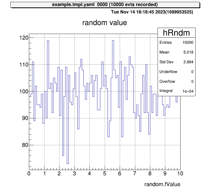
Next, let’s also check the histogram in “test2” directory and display two histograms vertically at the same time!
artemis [7] zone 2 1 # row=2, column=1
artemis [8] ht 0 # show the current hist
artemis [9] cd ..
artemis [10] ls

 artemis
>   0 art::TTreeProjGroup test2           test (2)
    1 art::TTreeProjGroup test            test
    2 art::TAnalysisInfo analysisInfo

artemis [11] cd 0

 test2
>   0 art::TH1FTreeProj hRndm2          random number

artemis [12] ht 0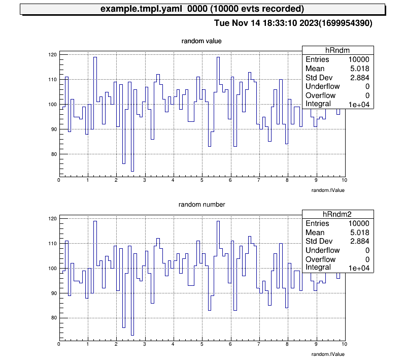
Now consider displaying a diagram from a TTree object. The file is created at here.
artemis [13] fls
 files
    0 TFile output/0001/example_0001.tree.root            (CREATE)
We use the fcd command to navigate to this root file.
artemis [14] fcd 0
artemis [15] ls

 output/0001/example_0001.tree.root
>   0 art::TAnalysisInfo analysisInfo
    1 art::TArtTree tree            tree
The command branchinfo (“br”) displays a list of the branches stored in this tree.
artemis [16] br
random               art::TSimpleData
At the same time, the ROOT command can be used.
artemis [17] tree->Print()
******************************************************************************
*Tree    :tree      : tree                                                   *
*Entries :    10000 : Total =          600989 bytes  File  Size =      86144 *
*        :          : Tree compression factor =   7.00                       *
******************************************************************************
*Br    0 :random    : art::TSimpleData                                       *
*Entries :    10000 : Total  Size=     600582 bytes  File Size  =      85732 *
*Baskets :        1 : Basket Size=    3200000 bytes  Compression=   7.00     *
*............................................................................*What is stored in the branch is not the usual type like “double” or “int”, but a class defined in artemis. Therefore, the “artemis” root file cannot be opened by usual ROOT.
Accessing data in a branch’s data class requires the use of public variables and methods, which can be examined by providing arguments to branchinfo [branch name] or classinfo [class name].
artemis [18] br random

 art::TSimpleData

 Data Members


 Methods

                   Bool_t   CheckTObjectHashConsistency
             TSimpleData&   operator=
             TSimpleData&   operator=

 See also

     art::TSimpleDataBase<double>

artemis [19] cl art::TSimpleDataBase<double>

 art::TSimpleDataBase<double>

 Data Members

                   double   fValue

 Methods

                     void   SetValue
                   double   GetValue
                   Bool_t   CheckTObjectHashConsistency
     TSimpleDataBase<double>&   operator=

 See also

     art::TDataObject       base class for data object
Therefore, it can be seen that it can be accessed by the value fValue.
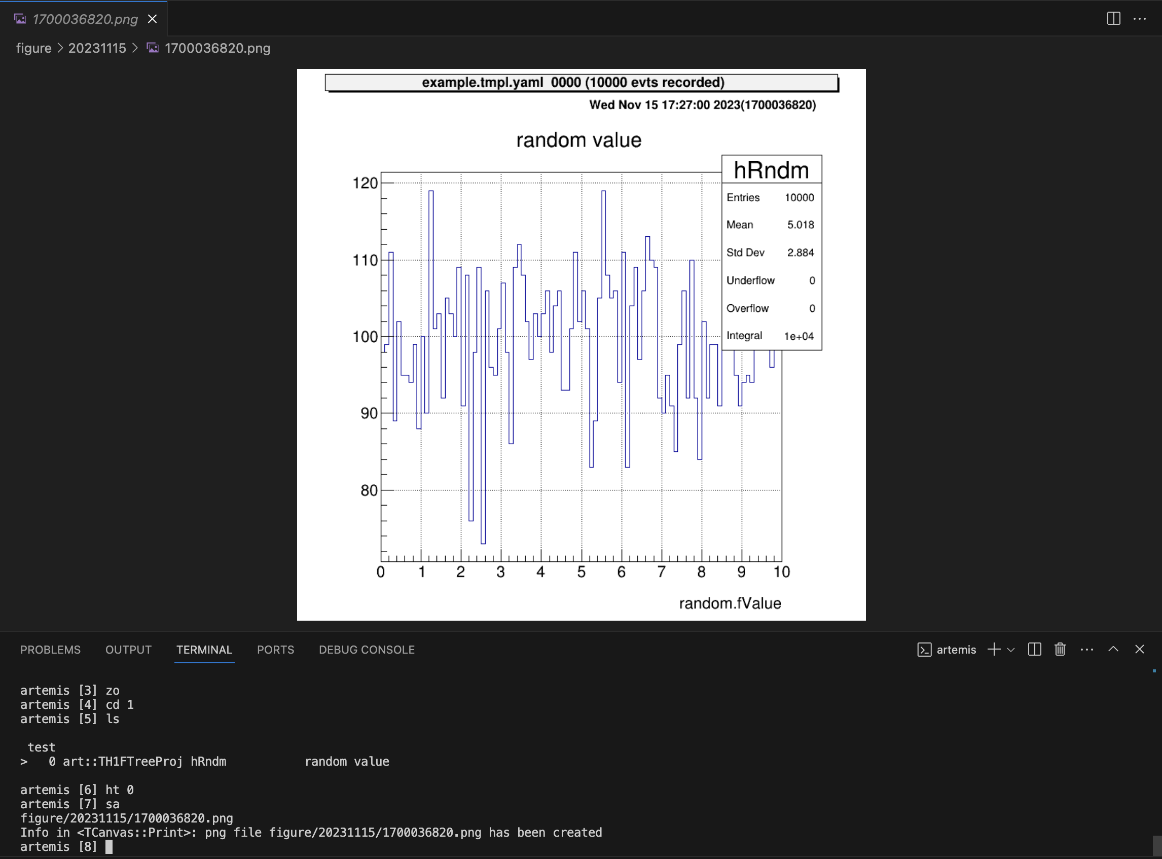
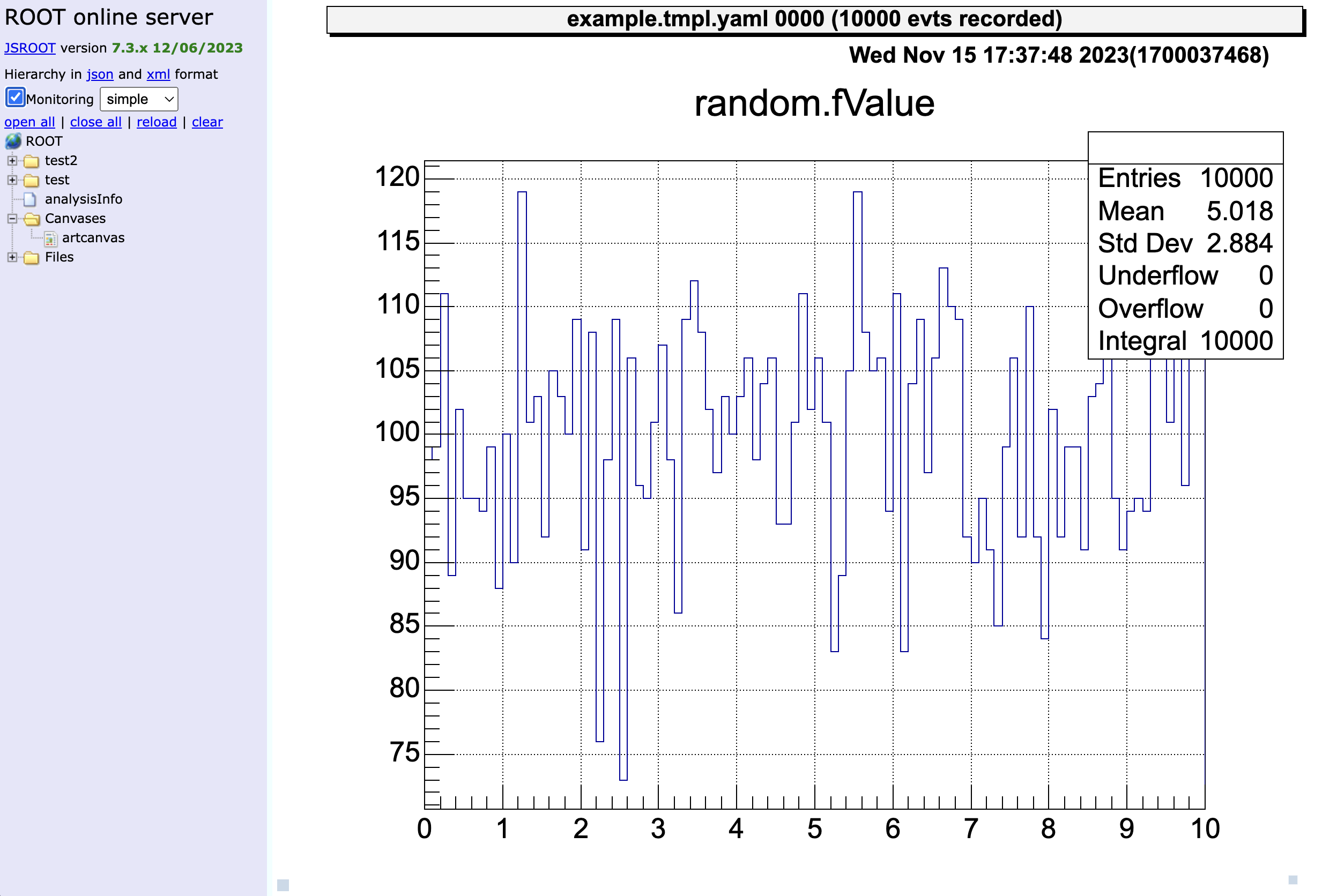
artemis [20] zone
artemis [21] tree->Draw("random.fValue>>(100,0.,10.)")artemis [*] help # show the commands we can use
artemis [*] save # save the current canvas
artemis [*] print # print the current canvas (send to the printer, need to configure)
artemis [*] unzoom
artemis [*] lgy, lgz, lny, lnz # linear or log scaleFrom this section, we start to configure the settings according to the actual experimental setup. The setting files are followings:
> tree
.
├── mapper.conf
├── conf
│   ├── map
│   │   ├── ppac
│   │   │   ├── dlppac.map

-- snip --

│   └── seg
│       ├── modulelist.yaml
│       └── seglist.yaml

-- snip --The data obtained from an ADC/TDC is in the form of, for example, “The data coming into channel 10 of an ADC with an ID of 1 is 100”.
---
title: Data flow example
---
graph LR;
    A{detector} -->|signal| B(TDC/ADC<br></br>ID=1, ch=10)
    B -->|value=100| C[<strong>Data build</strong>\nridf file]
The role of the map file is to map this value of “100” to an ID that is easy to analyse. An ID that is easy to analyse means, for example, that even if signals from the same detector are acquired with different ADCs/TDCs, the same ID is easier to handle in the analysis.
---
title: Data flow example
---
graph LR;
    A(TDC/ADC<br></br>ID=1, ch=10) -->|value=100| B[<strong>Data build</strong>\nridf file]
    B -->|value=100 mapping to| C(analysis<br></br>ID=2, ch=20)
After mapping, we can check the data of this “100” from ID=2 and ch=20. This ID and channel (2, 20) are provided for convenience, so you can freely set them.
So, in summary, the map file role is like this:
---
title: role of the map file
---
graph LR;
    A(DAQ ID<br></br>ID=1, ch=10) <-->|mapping| B(analysis ID<br></br>ID=2, ch=20)
CRIB is using Babirl for the DAQ system. In this system, the DAQ ID represented in the example is determined by five parameters.
The dev, fp, det and geo parameters can be set from DAQ setting. For the CRIB experiment, conventionally we set dev=12, fp=0–2 (for each MPV), det=6,7 (6=energy, 7=timing) and geo=from 0. But you can change it freely.
And analysis ID represented in the example is determined by two parameters.
Of cource you can also set the value freely.
The format of the map file is followings:
# [category] [id] [[device] [focus] [detector] [geo] [ch]] ....
1, 0, 12, 1, 6, 0, 0# map for SSD
# [category] [id] [[device] [focus] [detector] [geo] [ch]] ....
#
# Map: energy, timing
#
#--------------------------------------------------------------------
1, 0, 12, 1, 6, 0, 0, 12, 2, 7, 0, 0Please create map files for all detectors like this!
You can select the map file to be loaded with this file. This is especially useful when separating map files for testing from map files for the experiment.
The format is followings: (path/to/the/map/file number)
# file path for configuration, relative to the working directory
# (path to the map file) (Number of columns)
# cid = 1: rf
conf/map/rf/rf.map 1In the note example above, the number is 2.
Please do not forget to add to the mapper.conf after you add some map files.
This conf files are used when you use “chkseg.yaml” steering file. This steering file create raw data 2D histograms. I will describe in the Example: online_analysis/Check raw data in detail.
The steering file (yaml format) is a file that directs the process of how the obtained data is to be processed.
The artemis is an object-oriented program whose components are called processors, which are combined to process data.
The main role of the “processor” is to process data from an input data called InputCollection and create an output data called OutputCollection.
This “OutputCollection” will be stored into the root file as a “tree”.
Complex processing can be performed by using “processor” in multiple steps.
I will explain how to create this “steering” file using Si detector data as an example.
---
title: example of the data process structure
---
graph TD;
subgraph event loop
A-->B(mapping processor<br></br>InputCollection: decoded data\nOutputCollection: Si raw data)
B-->C(calibration processor<br></br>InputCollection: Si raw data\nOutputCollection: Si calibrated data)
C-->X((event end))
X-->A
end
subgraph DAQ
D(Raw binary data)-->A(decode processor<br></br>InputCollection: raw data\nOutputCollection: decoded data)
end
First, I describe what is the Anchor and how to use command line arguments.
See example here.
Anchor:
- &input ridf/@NAME@@NUM@.ridf
- &output output/@NAME@/@NUM@/chkssd@NAME@@NUM@.root
- &histout output/@NAME@/@NUM@/chkssd@NAME@@NUM@.hist.rootYou can use variables from elsewhere in the steering file by declaring them as such. For example if you write:
something: *inputThis unfolds as follows:
something: ridf/@NAME@@NUM@.ridfVariables enclosed in @ can also be specified by command line arguments.
For example, If you command like the following in the artemis console,
artemis [1] add steering/chkssd.yaml NAME=run NUM=0000it is considered as
Anchor:
- &input ridf/run0000.ridf
- &output output/run/0000/chkssdrun0000.root
- &histout output/run/0000/chkssdrun0000.hist.rootWhen using the “Babirl”, the data file will be in the form of “ridf”. In this case, the beginning and end of the steering file is usually as follows.
Processor:
- name: timer
type: art::TTimerProcessor
- name: ridf
type: art::TRIDFEventStore
parameter:
OutputTransparency: 1
InputFiles:
- *input
SHMID: 0
- name: mapper
type: art::TMappingProcessor
parameter:
OutputTransparency: 1
# -- snip --
- name: outputtree
type: art::TOutputTreeProcessor
parameter:
FileName:
- *outputEventStore (see below)OutputTransparency is set to 1, indicating that “OutputCollection” is not exported to the root file.
The “mapping processor” puts the data stored in the “EventStore” into a certain data class based on “mapper.conf”. Assume the following map file is used.
# map for SSD
# [category] [id] [[device] [focus] [detector] [geo] [ch]] ....
#
# Map: energy, timing
#
#--------------------------------------------------------------------
1, 0, 12, 1, 6, 0, 0, 12, 2, 7, 0, 0In this case, since we are assuming data from the Si detector, let’s consider putting it in a data class that stores energy and timing data, “TTimingChargeData”! The processor mapping to this data class is “TTimingChargeMappingProcessor”.
Processor:
- name: proc_ssd_raw
type: art::TTimingChargeMappingProcessor
parameter:
CatID: 1
ChargeType: 1
ChargeTypeID: 0
TimingTypeID: 1
Sparse: 1
OutputCollection: ssd_rawThen, you can access the ssd_raw data by using like tree->Draw("ssd_raw.fCharge")
While the data in the “ssd_raw” are raw channel of the ADC and TDC, it is important to see the data calibrated to energy and time. I will explain the details in Example: preparation/macro, but here I will discuss the calibration processors assuming that the following appropriate calibration files have been created.
Now, let’s load these files.
Processor:
- name: proc_ssd_ch2MeV
type: art::TParameterArrayLoader
parameter:
Name: prm_ssd_ch2MeV
Type: art::TAffineConverter
FileName: prm/ssd/ch2MeV.dat
OutputTransparency: 1
- name: proc_ssd_ch2ns
type: art::TParameterArrayLoader
parameter:
Name: prm_ssd_ch2ns
Type: art::TAffineConverter
FileName: prm/ssd/ch2ns.dat
OutputTransparency: 1To calibrate data contained in a TTimingChargeData class, a TTimingChargeCalibrationProcessor processor is used.
Processor:
- name: proc_ssd
type: art::TTimingChargeCalibrationProcessor
parameter:
InputCollection: ssd_raw
OutputCollection: ssd_cal
ChargeConverterArray: prm_ssd_ch2MeV
TimingConverterArray: prm_ssd_ch2nsNote here that “InputCollection”, “ChargeConverterArray”, and “TimingConverterArray” use the same names as the highlighted lines in the code block above.
The arguments to be used will vary depending on the processor used, so please check and write them according to the situation. If you want to check from artemis console, you can use “processordescription” command like this
> artlogin (username)
> a
artemis [0] processordescription art::TTimingChargeCalibrationProcessor
Processor:
- name: MyTTimingChargeCalibrationProcessor
type: art::TTimingChargeCalibrationProcessor
parameter:
ChargeConverterArray: no_conversion # [TString] normally output of TAffineConverterArrayGenerator
InputCollection: plastic_raw # [TString] array of objects inheriting from art::ITiming and/or art::ICharge
InputIsDigital: 1 # [Bool_t] whether input is digital or not
OutputCollection: plastic # [TString] output class will be the same as input
OutputTransparency: 0 # [Bool_t] Output is persistent if false (default)
TimingConverterArray: no_conversion # [TString] normally output of TAffineConverterArrayGenerator
Verbose: 1 # [Int_t] verbose level (default 1 : non quiet)If you want to analyse a large number of detectors, not just Si detectors, writing everything in one steering file will result in a large amount of content that is difficult to read.
In that case, we can use “include” node!
In the examples we have written so far, let’s only use a separate file for the part related to the analysis of the Si detector.
# -- snip --
Processor:
# -- snip --
- include: ssd/ssd_single.yaml
# -- snip --Processor:
# parameter files
- name: proc_ssd_ch2MeV
type: art::TParameterArrayLoader
parameter:
Name: prm_ssd_ch2MeV
Type: art::TAffineConverter
FileName: prm/ssd/ch2MeV.dat
OutputTransparency: 1
- name: proc_ssd_ch2ns
type: art::TParameterArrayLoader
parameter:
Name: prm_ssd_ch2ns
Type: art::TAffineConverter
FileName: prm/ssd/ch2ns.dat
OutputTransparency: 1
# data process
- name: proc_ssd_raw
type: art::TTimingChargeMappingProcessor
parameter:
CatID: 1
ChargeType: 1
ChargeTypeID: 0
TimingTypeID: 1
Sparse: 1
OutputCollection: ssd_raw
- name: proc_ssd
type: art::TTimingChargeCalibrationProcessor
parameter:
InputCollection: ssd_raw
OutputCollection: ssd_cal
ChargeConverterArray: prm_ssd_ch2MeV
TimingConverterArray: prm_ssd_ch2nsIn this way, the contents of “chkssd.yaml” can be kept concise, while the same process is carried out. Note that the file paths here are relative to the paths from the steering directory. Parameter files, for example, are relative paths from the working directory (one level down).
Utilising file splitting also makes it easier to check the steering files that analyse a large number of detectors like this.
# -- snip --
Processor:
# -- snip --
- include: rf/rf.yaml
- include: ppac/f1ppac.yaml
- include: ppac/dlppac.yaml
- include: mwdc/mwdc.yaml
- include: ssd/ssd_all.yaml
# -- snip --When you include other files, you can set arguments. This can be used, for example, to share variables. Details will be introduced in the example section.
The whole steering file is as follows:
Anchor:
 - &input ridf/@NAME@@NUM@.ridf
 - &output output/@NAME@/@NUM@/chkssd@NAME@@NUM@.root
 - &histout output/@NAME@/@NUM@/chkssd@NAME@@NUM@.hist.root
Processor:
- name: timer
type: art::TTimerProcessor
- name: ridf
type: art::TRIDFEventStore
parameter:
OutputTransparency: 1
InputFiles:
- *input
SHMID: 0
- name: mapper
type: art::TMappingProcessor
parameter:
OutputTransparency: 1
- include: ssd/ssd_single.yaml
# output root file
- name: outputtree
type: art::TOutputTreeProcessor
parameter:
FileName:
- *outputProcessor:
# parameter files
- name: proc_ssd_ch2MeV
type: art::TParameterArrayLoader
parameter:
Name: prm_ssd_ch2MeV
Type: art::TAffineConverter
FileName: prm/ssd/ch2MeV.dat
OutputTransparency: 1
- name: proc_ssd_ch2ns
type: art::TParameterArrayLoader
parameter:
Name: prm_ssd_ch2ns
Type: art::TAffineConverter
FileName: prm/ssd/ch2ns.dat
OutputTransparency: 1
# data process
- name: proc_ssd_raw
type: art::TTimingChargeMappingProcessor
parameter:
CatID: 1
ChargeType: 1
ChargeTypeID: 0
TimingTypeID: 1
Sparse: 1
OutputCollection: ssd_raw
- name: proc_ssd
type: art::TTimingChargeCalibrationProcessor
parameter:
InputCollection: ssd_raw
OutputCollection: ssd_cal
ChargeConverterArray: prm_ssd_ch2MeV
TimingConverterArray: prm_ssd_ch2ns> acd
> a
artemis [0] add steering/chkssd.yaml NAME=run NUM=0000In the online analysis, it is important to have immediate access to data. The artemis can produce TTree object but long commands are needed to access, for example,
artemis [1] fcd 0  # move to the created rootfile
artemis [2] zone 2 2  # make a "artemis" 2x2 canvas
artemis [3] tree->Draw("ssd_cal.fCharge:ssd_cal.fTiming>(100,0.,100., 100,0.,100)","ssd_cal.fCharge > 1.0","colz")
This would take time if there are some histograms that you want to display immediately…
Therefore, if you know in advance the diagram you want to see, it is useful to predefine its histogram!
The processor used is TTreeProjectionProcessor.
I would like to explain how to use this one.
Let’s look at how histograms are defined when looking at SSD data. First, let’s prepare the steering file as follows! please see previous section for omissions.
# -- snip --

  - include: ssd/ssd_single.yaml

# Histogram
  - name: projection_ssd
    type: art::TTreeProjectionProcessor
    parameter:
      FileName: hist/ssd/ssd.yaml
      Type:     art::TTreeProjection
      OutputFilename: *histout


# output root file
  - name: outputtree
    type: art::TOutputTreeProcessor
    parameter:
      FileName:
        - *output
The histogram is created based on the TTree object,
so describe the processing of the histogram after the part that represents the data processing and before the part that outputs the TTree (TOutputTreeProcessor).
There are three points to note here.
Therefore, I would now like to show the histogram definition file.
First please look at this example.
 1anchor:
 2  - &energy ["ssd_cal.fCharge",100,0.,100.]
 3  - &timing ["ssd_cal.fTiming",100,0.,100.]
 4alias:
 5  energy_cut: ssd_cal.fCharge>1.0;
 6group:
 7  - name: ssd_test
 8    title: ssd_test
 9    contents:
10      - name: ssd_energy
11        title: ssd_energy
12        x: *energy
13
14      - name: ssd_timing
15        title: ssd_timing
16        x: *timing
17
18      - name: ssd_energy and timing
19        title: ssd_energy and timing
20        x: *timing
21        y: *energy
22        cut: energy_cut
This definition file consists of three parts.
The actual core part is the “2.3 group”, but “2.1 anchor” and “2.2 alias” are often used to make this part easier to write.
The anchor defines the first argument of tree->Draw("ssd_cal.fCharge>(100,0.,100.)","ssd_cal.fCharge > 1.0")
The array stored in the variable named “energy” in the second line looks like [str, int, float, float] and has the following meanings
As you might imagine, inside the first argument you can also add operations such as TMath::Sqrt(ssd_cal.fCharge) or ssd_cal.fCharge-ssd_cal.fTiming, because it is the same with “tree->Draw”.
Note, however, that the definition here is for one-dimensional histograms. Two-dimensional histograms will be presented in Section 2.3. It is very simple to write!
This part is used when applying gates to events (often we call it as “cut” or “selection”).
For example, if you only want to see events with energies above 1.0 MeV, you would write something like tree->Draw("energy","energy>1.0").
The alias node is used to define the part of energy>1.0
A semicolon “;” at the end of the sentence may be needed…? please check the source.
The histogram is defined here and the object is stored in a directory in artemis (ROOT, TDirectory). In the example shown above, the directory structure would look like this:
(It is not actually displayed in this way).
# in artemis
.
└── ssd_test
    ├── ssd_energy (1D hist)
    ├── ssd_timing (1D hist)
    └── ssd_energy and timing (2D hist)
The first “name” and “title” nodes are arguments of TDirectory instance. Also the second “name” and “title” nodes are arguments of instance of TH1 or TH2 object. The other “x”, “y” and “cut” is the important node!
There are many useful command for checking the histogram objects. These are similar to the ANAPAW commands.
> artlogin (username)
> a

artemis [0] add steering/chkssd.yaml NAME=hoge NUM=0000
artemis [1] res
artemis [2] sus
artemis [3] ls # check the artemis directory

 artemis
>   0 art::TTreeProjGroup ssd_test        ssd_test
1 art::TAnalysisInfo analysisInfoartemis [4] cd 0
artemis [5] ls
ssd_test
> 0 art::TH1FTreeProj ssd_energy ssd_energy
1 art::TH1FTreeProj ssd_timing ssd_timing
2 art::TH2FTreeProj ssd_energy and timing ssd_energy and timingartemis [6] ht 0
artemis [7] ht 2 colzWhen setting up several detectors of the same type and wanting to set up a histogram with the same content, it is tedious to create several files with only the names of the objects changed. In such cases, it is useful to allow the histogram definition file to have arguments.
Please look here first.
# -- snip --

  - include: ssd/ssd_single.yaml

# Histogram
  - name: projection_ssd
    type: art::TTreeProjectionProcessor
    parameter:
      FileName: hist/ssd/ssd.yaml
      Type:     art::TTreeProjection
      OutputFilename: *histout
      Replace: |
        name: ssd_cal

# -- snip --
We add the highlighted lines.
Then the “name” can be used at hist file by @name@!
The “name” can be freely set.
anchor:
  - &energy ["@name@.fCharge",100,0.,100.]
  - &timing ["@name@.fTiming",100,0.,100.]
alias:
  energy_cut: @name@.fCharge>1.0;
group:
  - name: ssd_test
    title: ssd_test
    contents:
      - name: ssd_energy
        title: ssd_energy
        x: *energy

      - name: ssd_timing
        title: ssd_timing
        x: *timing

      - name: ssd_energy and timing
        title: ssd_energy and timing
        x: *timing
        y: *energy
        cut: energy_cut
This is useful when there are more objects to check!
# -- snip --

  - include: ssd/ssd_single.yaml

# Histogram
  - name: projection_ssd
    type: art::TTreeProjectionProcessor
    parameter:
      FileName: hist/ssd/ssd.yaml
      Type:     art::TTreeProjection
      OutputFilename: *histout
      Replace: |
        name: ssd_cal

  - name: projection_ssd
    type: art::TTreeProjectionProcessor
    parameter:
      FileName: hist/ssd/ssd.yaml
      Type:     art::TTreeProjection
      Replace: |
        name: ssd_raw
  # and so on!

# -- snip --
File splitting using “include” nodes, as described in the section on steeling, can also be used in the same way.
When we start the analysis, there are many situations where the analysis server on which artemis is installed is not only operated directly, but also remotely using “ssh”.
In such cases, there are various settings that need to be made in order for the figure to be displayed on the local computer, and some of these methods are described in this section.
We recommended to use VNC server currently, but note that policies may change in the future.
This is a list of ways to display the figures.
This is the simplest method. Simply transfer the remote X to the local.
ssh -X analysisPCThis “X” option allow the X11Forwarding.
However, the problem with this method is that it takes a long time to process, and it takes longer from the time the command is typed until it is drawn. It is also not recommended as the process can become slow if a large number of people use it at the same time.
However, it is simpler than other methods and should be used when necessary, e.g. for debugging.
This is old version of VNC server (TigerVNC). Latest version supports more secure method, so this method may no longer be avaliable in the future…
First please install VNC viewer to your PC. Any viewer may work well, but we are using this software.
First, please check the ID number of the VNC server we are running.
> vncserver -list

TigerVNC server sessions:

X DISPLAY #	PROCESS ID
:1		  3146
:5		  7561
:2022	  29499
:2		  23055
In this example, number 1, 5, 2022 and 2 VNC server is running. And select an available number to start the VNC server you want to use.
> vncserver :10 # start the VNC server!If you want to kill the VNC server, the below command will work.
> vncserver -kill :10 # kill the VNC server!Next, configure the canvas created by artemis to be sent to a VNC server.
The a command can treat this process by using .vncdisplay file!
> artlogin (username) # move to your artemis work directory
> echo "10" > .vncdisplay # write the ID of VNC server to the .vncdisplay file
Then, the setting in analysis PC is completed! The next step is to set up your local PC to receive this.
If you connect your PC in the same network with analysis PC, you can directory connect using the VNC viewer. However, CRIB analysis PC are connected CNS local network. In order to connect from outside network, we need to use “CNS login server”. If you want to make the login server account, please contact the CRIB member!
In this section, we are assuming that you have a CNS login server account.
To access the analysis PC, use two-stage ssh. Prepare the following configuration file.
Host login
    # need to change
    HostName CNS_loginserver_hostname
    User username
    IdentityFile ~/.ssh/id_rsa
    # no need to change (if you want)
    ForWardX11Timeout 24h
    ControlPersist 30m
    ForwardAgent yes
    ControlMaster auto
    ControlPath ~/.ssh/mux-%r@%h:%p

# any name is okay
Host analysis
    # need to change
    HostName analysisPC_hostname
    User username
    IdentityFile ~/.ssh/id_rsa
    # no need to change (if you want)
    ProxyCommand ssh login nc %h %p
    ForwardAgent yes
    ControlMaster auto
    ControlPath ~/.ssh/mux-%r@%h:%p
    ControlPersist 30m
Then you can access to the analysis PC simply by:
> ssh analysisNext, in order to receive from the VNC server, we use port-forwarding! VNC servers with ID x use port number 5900+x. For example if we use number “10”, the port will be 5910.
Forward this to a certain port on localhost. This number can be any number that is not in use.
---
title: An example of port-forwarding
---
graph LR;
    A(analysis PC<br></br>port 5910) --> |send|B(local PC<br></br>port 55910)
Host analysis
    HostName analysisPC_hostname
    User username
    IdentityFile ~/.ssh/id_rsa
    LocalForward 55910 localhost:5910
    ProxyCommand ssh login nc %h %p
    ForwardAgent yes
    ControlMaster auto
    ControlPath ~/.ssh/mux-%r@%h:%p
    ControlPersist 30m
This allows you to display a VNC display by accessing port 55910 on your own PC (localhost), instead of having to access port 5910 on the analysis PC!
If your PC is in the same network, changing “localhost” to the “IP address of analysis PC” is okay (ex. 192.168.1.10:5910).
VScode is very exciting editor! The extension supports ssh and allows remote png files to be displayed on the editor.
However, it is a bit time-consuming as the diagram has to be saved each time to view it. Please refer to this as one method.
This is option…
Now the histogram object cannot display by JSROOT, because the object is not actually “TH1” or “TH2” object but “TH1FTreeProj” or “TH2FTreeProj”. (ref: issue#40)
We can only display the “TCanvas” Object.
Artemis configuration varies from experiment to experiment. We would like to explain in this chapter how they are configured and used in CRIB experiment.
CRIB shares the analysis environment of all experiments under one user account (username crib). Therefore, when you want to check data from an old experiment or when several people are analysing the data, you need to log in to the same user account.
Of course, the analysis environment varies according to the experiment (and even different environments for different users within the same experiment!) and these have to be managed well. The “.bashrc/.zshrc” and “artlogin (artlogin2)” commands set them up. Currently we are using “zsh (.zshrc)”.
export EXP_NAME="current" # your experiment
export EXP_NAME_OLD="previous" # old experiment
The EXP_NAME is current experiment and you can enter the environment by using artlogin command.
At the same time, the EXP_NAME_OLD is the old experiment and you can use artlogin2 command.
In the current version, we support two experimental environment and if you want to check other experimental data, please change EXP_NAME_OLD.
When you modify “.bashrc/.zshrc”, all people’s settings will change.
Therefore please do not change EXP_NAME as much as possible, because we want to set this environment variable as the active experiment.
If you change this, please report it so that CRIB members are aware of it.
Commands may be created in the future to enter the environment of all experiments flexibly, not just two. (like artoldlogin {expname} {username}?)
Then you can enter the different analysis environment like this:
> artlogin (username)
> artlogin2 (username)CRIB uses a default user as well as individual analysis environments. The username of the default user is the same with experiment name.
If you set the name of the experiment to “si26a” (EXP_NAME), then the username “si26a” will be the default user.
The user’s environment can be entered with the “artlogin” command with no arguments.
> artlogin
> pwd
/home/crib/art_analysis/si26a/si26a
If you want to test something by changing files, or if you want to use your own VNC server, you can enter that environment by specifying its name as an argument.
> artlogin okawa # if this is the first time to command, you will see setup comments.
> pwd
/home/crib/art_analysis/si26a/okawaWhen using the default user, try to avoid using a VNC server (do not create .vncdisplay files). The main reason for creating a default user is to analyse locally (for shifters) in the online analysis, and using a VNC server makes it impossible to view the figures locally.
The directory structure comprising artemis is as follows. (The location of artemis itself is omitted).
> tree -L 2 ~/art_analysis
/home/crib/art_analysis
├── current # accessed by "artlogin"
│   ├── current # default user
│   └── okawa # individual user
├── previous # accessed by "artlogin2"
│   ├── previous
│   └── okawa
├── old1
│   ├── old1
│   └── okawa
└── old2

# -- snip --We often use “nssta” (non-save mode start) analysis in the beam tuning.
It is not necessary to take data, but we need to check the beam condition by using artemis.
In this case, TRIDFEventStore can be used as online mode.
By default, if we don’t add an input file name and set the SHMID (Shared Memory ID), artemis will use online mode. However, it is necessary to use different types of steering files, one for use in online-mode and the other for use from a file, which can be complicated…
Therefore, the same steering file was changed to automatically go online mode when the ridf file was not present.
# from ridf files
artemis [0] add steering/hoge.yaml NAME=hoge NUM=0000
# online-mode
artemis [0] add steering/hoge.yaml # no argumentTo achieve this, the original file was changed as follows.
129    for (Int_t i=0; i!=n;i++) {
130       printf("file = %s\n",fFileName[i].Data());
131+      if(!gSystem->FindFile(".", fFileName[i])) {
132+         Info("Init", "No input file -> Online mode");
133+         fIsOnline = kTRUE;
134+      }
135    }
We always use SHMID=0, so it works simply by adding the following sentence.
   - name: ridf
     type: art::TRIDFEventStore
     parameter:
       OutputTransparency: 1
       InputFiles:
         - *input
SHMID: 0still under consideration in this part!
CRIB often wants to customise artemis because it originally used ANAPAW and wants to perform analysis like ANAPAW. However, we do not want to make too many changes to the source code of artemis itself, and we want to make it work in the user-defined part. (it means in the artemis work directory)
In particular, it is often the case that we want to create a new artemis command, but writing the command source on the work directory and registering it in artemislogon.C did not work somehow…
Also, artemislogon.C is automatically generated (from .artemislogon.C.in) by the cmake functionality, and even if this itself is changed, it will revert when cmake is redone.
Therefore, a file called userlogon.C was prepared, which only took out the user-defined part from artemislogon.C.
The following files have been modified to read this.
14 #include <TInterpreter.h>
15+#include <TSystem.h>
16 #include "TLoopManager.h"
44    TRint::ProcessLine(".x artemislogon.C");
45+   FileStat_t info;
46+   if (gSystem->GetPathInfo("userlogon.C", info)==0) {
47+      TRint::ProcessLine(".x userlogon.C");
48+   }
If there is a userlogon.C file in the work directory, it is loaded, otherwise artemis can be used as usual.
This file can be used freely! What we wanted to do most is to register user-defined commands, which can be done as follows.
{
   // load user function
   gROOT->ProcessLine(".L macro/UserUtil.C");

   // User commands register
   // cf definition: TCatCmdFactory *cf = TCatCmdFactory::Instance();
   cf->Register(TCatCmdLoopStart::Instance());
   cf->Register(TCatCmdLoopStop::Instance());
   cf->Register(new art::TCmdXfitg);
   cf->Register(new art::TCmdXstatus);
   cf->Register(new art::TCmdXYblow);
   cf->Register(new art::TCmdXblow);
   cf->Register(TCatCmdTCutG::Instance());
   cf->Register(new art::TCmdErase);
   cf->Register(new art::TCmdDraw);

   // TTree merge setting
   TTree::SetMaxTreeSize( 1000000000000LL ); // 1TB
}
The first line gROOT->ProcessLine(".L macro/UserUtil.C") load the user definition function.
You can add any function to the “macro/UserUtil.C” file, and the function to load TCutG object in “/gate/*.root” directory is written defaultly.
For more detail, please see tcutg command and gate pages.
(For some reason, an error occurred when writing in artemislogon.C.) You can also customise it in other ways to make it easier for you. For example, when creating a TTree, a setting to increase the file size limit is also included by default.
Various commands (mainly the same with ANAPAW commands) have been developed for CRIB experiment. For more information, please click here (src-crib/commands). These commands are registered in userlogon.C. (See previous section.)
This section explains how to use them.
the default figures:

This is exactly the same as the resume command, because ANAPAW starts the event loop with start instead of resume.
This is exactly the same as the suspend command, because ANAPAW stops the event loop with stop instead of suspend.
For 1D histograms, by selecting the two ends of two points, the peak between them is fitted with a Gaussian.
artemis [7] xf
Info in <art::TCmdXfitg::Cmd>: click on the lowest edge:
Info in <art::TCmdXfitg::Cmd>: click on the highest edge:
Info in <art::TCmdXfitg::Cmd>: X1: -1437.56, X2: -1419.11
 FCN=81.6642 FROM MIGRAD    STATUS=CONVERGED      71 CALLS          72 TOTAL
                     EDM=3.35095e-09    STRATEGY= 1      ERROR MATRIX ACCURATE
  EXT PARAMETER                                   STEP         FIRST
  NO.   NAME      VALUE            ERROR          SIZE      DERIVATIVE
   1  Constant     1.16439e+03   2.43862e+01   8.08454e-02   9.04256e-07
   2  Mean        -1.43081e+03   4.54001e-02   6.82262e-04  -1.74034e-03
   3  Sigma        2.81435e+00   4.07888e-02   1.55351e-05  -3.15946e-03
artemis [8]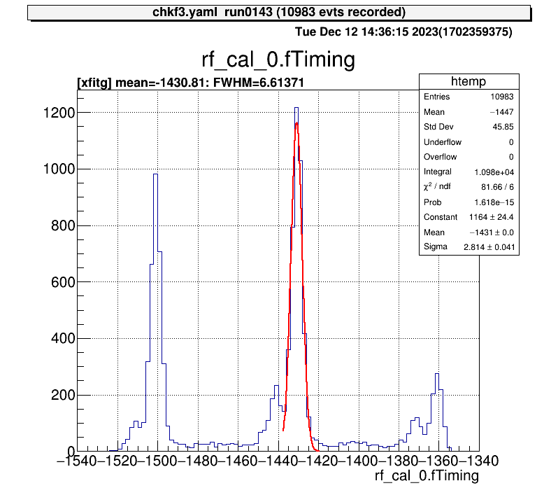
For 1D histograms, select both ends and crop the histogram between them.
artemis [10] xblo
Info in <art::TCmdXblow::Run>: click on the lowest edge:
Info in <art::TCmdXblow::Run>: click on the highest edge:
Info in <art::TCmdXblow::Run>: X1: -1439.3, X2: -1417.37
Info in <art::TCmdXblow::Run>: id = 2 hist is created
artemis [11]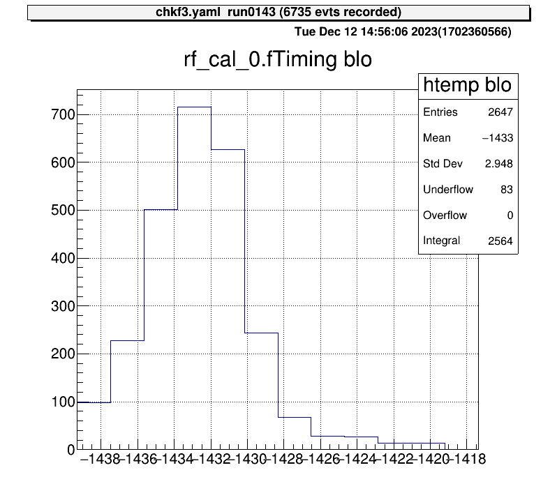
For 2D histograms, select both corners and crop the histogram between them.
artemis [60] xyblo
Info in <art::TCmdXYblow::Run>: click on one corner:
Info in <art::TCmdXYblow::Run>: X1: 9.2154, Y1: 46.6159
Info in <art::TCmdXYblow::Run>: click on the other corner:
Info in <art::TCmdXYblow::Run>: X2: 21.7032, Y2: 23.952
Info in <art::TCmdXYblow::Run>: id = 6 hist is created
artemis [61]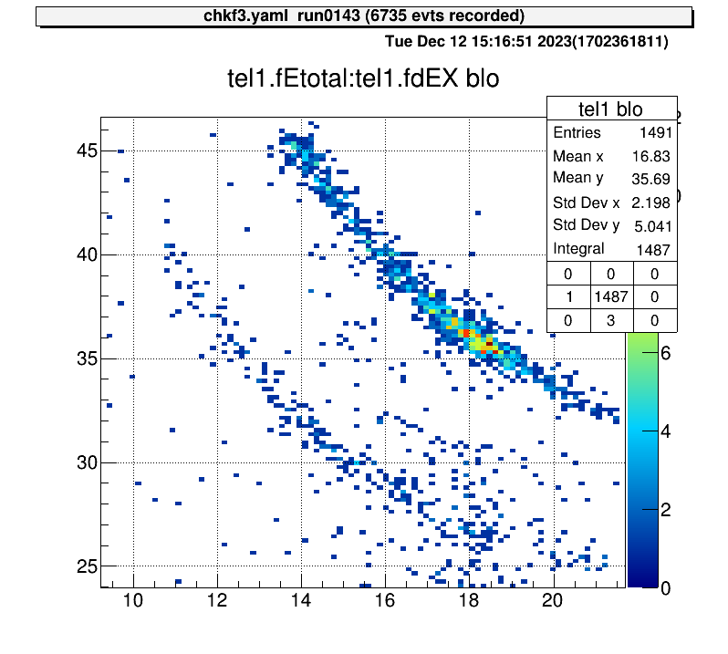
For 2D histograms, select both corners and determine the ratio of the total number of events.
artemis [8] xs
Info in <art::TCmdXstatus::Cmd>: click on one corner:
Info in <art::TCmdXstatus::Cmd>: X1: 14.1496, Y1: 41.4826
Info in <art::TCmdXstatus::Cmd>: click on the other corner:
Info in <art::TCmdXstatus::Cmd>: X2: 21.0941, Y2: 31.9909
------------------
selected = 976, total = 7526
ratio  = 0.129684 (12.9684%)
artemis [9]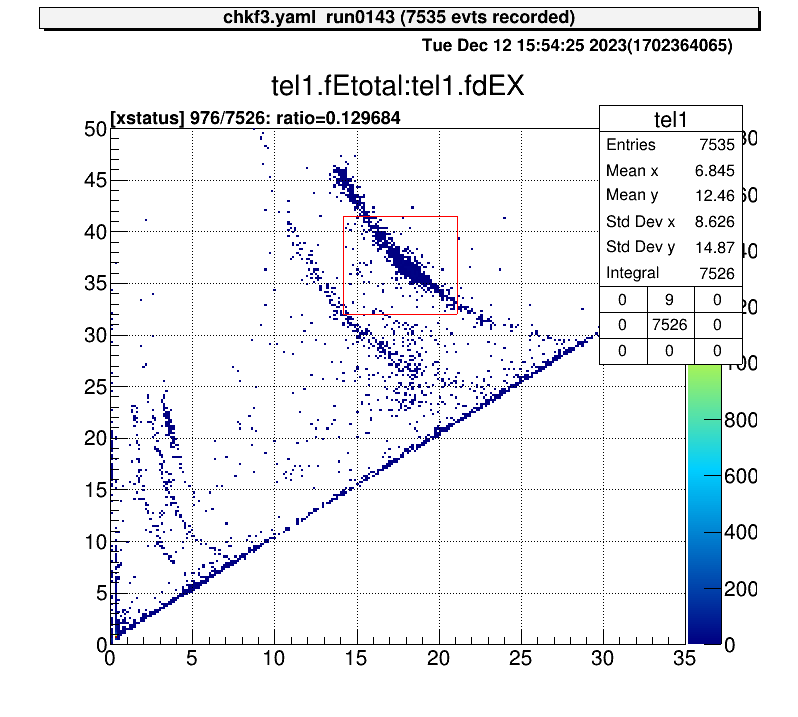
For 2D histograms, this command create TCutG object and store in a ROOT file.
If you select to save the object, the file will place to the gate/*.root directory.
There objects are automatically loaded. (please check user config page.)
This is the example how to use this command.
artemis [] ht something
artemis [] tc
Info in <TCatCmdTCutG::Cmd>: Xaxis name : f2ppac.fX  Yaxis name : f2ppac.fY
Info in <TCatCmdTCutG::Cmd>: When you have finished specifying the area (last point), double-click on it.
Info in <TCatCmdTCutG::Cmd>: (x, y) = (9.050404, 10.301410)
Info in <TCatCmdTCutG::Cmd>: (x, y) = (5.047341, -8.294592)
Info in <TCatCmdTCutG::Cmd>: (x, y) = (-12.183236, -3.839300)
Info in <TCatCmdTCutG::Cmd>: (x, y) = (3.306878, -15.074384)
Info in <TCatCmdTCutG::Cmd>: (x, y) = (-3.306878, -32.120720)
Info in <TCatCmdTCutG::Cmd>: (x, y) = (9.920635, -15.461801)
Info in <TCatCmdTCutG::Cmd>: (x, y) = (18.274854, -29.989928)
Info in <TCatCmdTCutG::Cmd>: (x, y) = (16.186299, -11.200217)
Info in <TCatCmdTCutG::Cmd>: (x, y) = (35.157338, -4.420425)
Info in <TCatCmdTCutG::Cmd>: (x, y) = (14.271791, -4.807841)
Info in <TCatCmdTCutG::Cmd>: (x, y) = (10.964912, 9.332869)
Info in <TCatCmdTCutG::Cmd>: (x, y) = (10.964912, 9.332869)
if you want to save it, input the TCutG name [name/exit] f2star
Info in <TCatCmdTCutG::Cmd>: Created gate/f2star.root
To select an area, click on the vertices of the area you want to select, then double-click at the last vertex.
If you want to save this object, enter the “cut” name.
In this example, I input the f2star as the object name.
If you don’t want to save, enter “exit”.
Then the gate/f2star.root will be created.
And after reload the artemis, the gate will be loaded automatically and we can use histogram definition and “tree->Draw” selection part.
For the detail please check gate page.
artemis [] tree->Draw("f2ppac.fY:f2ppac.fX>>(200,-50.,50., 200,-50.,50.)","f2star","colz")
Grammar issue I think.
 export LD_LIBRARY_PATH=$TARTSYS/lib:$LD_LIBRARY_PATH

-if [ "@BUILD_GET@" == "ON" ]; then
+if [[ "@BUILD_GET@" == "ON" ]]; then
     export LD_LIBRARY_PATH=@GET_LIB_DIR@:$LD_LIBRARY_PATH
 fi

-if [ "@MPI_CXX_FOUND@" == "TRUE" ]; then
+if [[ "@MPI_CXX_FOUND@" == "TRUE" ]]; then
     dir=@MPI_CXX_LIBRARIES@
     libdir="$(dirname $dir)"
Add cross hair.
84 void TCatCmdXval::GetEvent()
85 {
86+   dynamic_cast<TPad *>(gPad)->DrawCrosshair();
87    const int event = gPad->GetEvent();
After the command, the projected histogram will automatically be displayed.
55       if (!obj->InheritsFrom(TH2::Class())) {
56          // TArtCore::Info("TCatCmdPr::Run","%s is not 2D histogram",
57          //               obj->GetName());
58+        Info("Run", "%s is not 2D histogram", obj->GetName());
59          continue;
60       }
61+      Int_t nid = (gDirectory->GetList())->GetEntries();
62       Run((TH2*) obj, opt);
63+      Info("Run", "id = %d hist is created", nid);
64+      TCatHistManager::Instance()->DrawObject(nid);
65    }
66    return 1;
67 }
In the CRIB processor, there is a processor that inherits from TModuleInfo, TModuleData.
In the constractor of this class use copy constractor of TModuleInfo, but the default artemis doesn’t implement it.
This class is used when we want to check the raw data.
For the detail, please see check raw data page.
Therefore, we modified this like this:
31  TModuleInfo::TModuleInfo(const TModuleInfo& rhs)
32+   : TParameterObject(rhs),
33+   fID(rhs.fID),
34+   fType(rhs.fType),
35+   fHists(nullptr)
36  {
37+   if (rhs.fHist) {
38+     fHists = new TObjArray(*(rhs.fHists));
39+   }
40+
41+   fRanges = rhs.fRanges;
42  }
Up to now, we have introduced the installation and concepts of artemis. This chapter will show you how to analyse with artemis through practical examples; if you want to know how to use artemis, it is no problem to start reading from here.
This section explain the example of preparation by using some useful macro.
I would now like to introduce the actual analysis using the CRIB analysis server. There are two ways to enter the analysis server, directly or remotely via ssh. If you come to CRIB and operate the server directly, I think it is quicker to analyse using the server while asking the CRIB members directly as I think they are nearby.
To enter the CRIB server, you need to enter the CNS network. To do this, you need to create an account on the CNS login server. Please contact Okawa (okawa@cns.s.u-tokyo.ac.jp) or the person responsible for CRIB (see here) and tell us that you want a login server account.
The CNS login server uses public key cryptography, so you need to send a shared key when you apply. This section describes how to create the key, especially on MacOS.
cd # move to /Users/yourname/ (home directory)
mkdir .ssh # if there is no .ssh directory
cd .ssh
ssh-keygen
You will be asked a number of interactive questions after this command, all of which are fine by default (Enter). Then you will see the pair of public-key and private-key.
ls
id_rsa  id_rsa.pub
id_rsa is the private-key, and id_rsa.pub is the public-key.
The private key is important for security reasons and should be kept on your own computer.
Then, please send this public-key to the CNS member.
in MacOS, open . command will open a finder for that directory, so it is easy to attach it to an email from here.
In the email,
are needed.
Next, let’s set up multi-stage ssh. As the login server is just a jump server, it is useful to be able to ssh to the CRIB analysis server at once! So create the following config file. The file placed in this directory is automatically read when you ssh.
cd ~/.ssh
vi config 1Host login
2 HostName CNS_loginserver_hostname
3 User username
4 IdentityFile ~/.ssh/id_rsa
5 ForWardX11Timeout 24h
6 ControlPersist 30m
7 ForwardAgent yes
8 ControlMaster auto
9 ControlPath ~/.ssh/mux-%r@%h:%p
10
11# any name is okay
12Host cribana
13 HostName analysisPC_hostname
14 User crib
15 IdentityFile ~/.ssh/id_rsa
16 ProxyCommand ssh login nc %h %p
17 ForwardAgent yes
18 ControlMaster auto
19 ControlPath ~/.ssh/mux-%r@%h:%p
20 ControlPersist 30mYou will be informed of the second and third lines above that we highlighted, so please change this parts. And ask the IP address of the CRIB analysis PC to the CRIB member, and change the 13 line.
Then you can enter the CRIB analysis PC just by
ssh cribanaCRIB member will tell you the passward!
For the VNC server (local forwarding), please see this section.
When you enter the CRIB computer, please check this is zsh shell.
> echo $SHELL
/usr/local/bin/zshCurrently, zsh installed locally is used. It is planned to update the OS in the future, after which it will differ from this path in the future.
If it is not zsh (like bash), please command
> zshThen you can start to configure by
> artlogin yourname
# input your information...

> mkdir build
> cd build
> cmake ..
> make -j4
> make install
> acd
For the detail, please check here.
> acd # move to your artemis work directory
> a # start artemis!

> a macro/macro.C # run macro script# read steering file
artemis [*] add steering/hoge.yaml NAME=hoge NUM=0000
# start event loop
artemis [*] res
artemis [*] start # defined in CRIB artemis
# stop event loop
artemis [*] sus
artemis [*] stop # defined in CRIB artemis
# help
artemis [*] help
# quit from artemis
artemis [*] .q# check and move the directory
artemis [*] ls
artemis [*] cd 0 # cd ID
# move to home directory in artemis
artemis [*] cd # cd .. will work?
# draw the histograms
artemis [*] ht 0 colz # ht ID option
artemis [*] hn colz # draw the next histogram object
artemis [*] hb colz # draw the previous histogram object
# divide the canvas
artemis [*] zone 2 2 # 2 x 2 canvas
# save and print the canvas
artemis [*] sa
artemis [*] pri# check the files
artemis [*] fls
# move to the created ROOT file
artemis [*] fcd 0 # fcd fileID
# check the all branches
artemis [*] br
# check the data members or methods
artemis [*] br branchname # ex. artemis [1] br ppaca
# the name of TTree object is "tree" (actually TArtTree object)
artemis [*] tree->Draw("ppaca.fY:ppaca.fX>>ppaca(100,-20.,20., 100,-20.,20.)","","colz")See here for an example using random numbers.
CRIB uses a multi-hit TDC called V1190 to take timing data (manual). When a trigger comes into this module, it opens a window with a set time width and records the timing of the data.
However, even if the signal is sent at exactly the same time to the trigger, due to the uncertainty in opening that window, the resulting channel will vary. Since absolute channel values will vary, but relative channel values for a given (especially trigger) timing will remain the same, it is necessary to subtract all data by some reference channel to achieve good timing resolution.
The signal that serves as the reference for that time is what we call Tref!
(Time reference)
Since it is essential that all events contain that data, we put the trigger signal in one of the channels and make it a Tref.
The “tref” settings are made in the following file:
Processor:
# J1 V1190A
  - name: proc_tref_v1190A_j1
    type: art::TTimeReferenceProcessor
    parameter:
      # [[device] [focus] [detector] [geo] [ch]]
      RefConfig: [12, 2,  7, 0, 15]
      SegConfig: [12, 2,  7, 0]
Parameters RefConfig and SegConfig are set using the same ID as in the map file.
The “RefConfig” represents the “Tref” signal and the “SegConfig” represents the V1190 module. Therefore, the role of the processor is to subtract the “Segconfig” V1190 all timing signal from the “RefConfig” tref signal.
To apply this processor, add the following line to the steering file. For example,
Anchor:
 - &input ridf/@NAME@@NUM@.ridf
 - &output output/chkf3@NAME@@NUM@.root
 - &histout output/chkf3@NAME@@NUM@.hist.root

Processor:
  - name: timer
    type: art::TTimerProcessor

  - name: ridf
    type: art::TRIDFEventStore
    parameter:
      OutputTransparency: 1
      InputFiles:
        - *input

  - name: mapper
    type: art::TMappingProcessor
    parameter:
      OutputTransparency: 1

  - include: tref.yaml
  - include: rf/rf.yaml
  - include: coin/coin.yaml
  - include: ppac/dlppac.yaml
  - include: ssd/f3ssd.yaml

  - name: outputtree
    type: art::TOutputTreeProcessor
    parameter:
      FileName:
- *outputThe tref.yaml should be written before the main processor. In this example, it is written right after TMappingProcessor, and we recommend writing it in this position.
CRIB use two kinds of PPAC (Parallel-Plate Avalanche Counter), charge division method or delay-readout method. The PPAC placed at the F1 focal plane is charge-devision type, and the parameters to be converted to position are fixed and do not need to be calibrated. Therefore we explain the calibration method for delay-line PPAC (dl-PPAC).
Here we briefly describe the principle of converting from the obtained signal to position, but for more details, see here1.
We will discuss the x-direction because x and y is exactly same. First, define the parameters as follows
The artemis codes calculate the X position like this formula (see TPPACProcessor.cc).
$$ X~\mathrm{[mm]} = k_x\left( \frac{T_{X1} - T_{X2} + T_{Xin-offset} - T_{Xout-offset}}{2} \right) - X_{offset}$$Check the sign carefully! We often mistook the direction!!
The $T_{X1},~T_{X2}$ are measured value by TDC, and $k_x$ and $T_{Xin-offset}$ are specific value to PPAC, so we need to care only $T_{Xout-offset}$ and $X_{offset}$. $X_{offset}$ value depends on where we put the PPAC, so what we have to do is determine the line calibration parameter ( $T_{Xout-offset}$).
The following is a list of dl-PPAC parameters used in CRIB experiment.
| PPAC ID | $k_x$ [mm/ns] | $k_y$ [mm/ns] | $T_{Xin-offset}$ | $T_{Yin-offset}$ |
|---|---|---|---|---|
| #2 | 1.256 | 1.256 | 0.29 mm | 0.18 mm |
| #3 | 1.264 | 1.253 | 0.22 mm | 0.30 mm |
| #7 | 1.240 | 1.242 | 0.92 ns | 1.58 ns |
| #8 | 1.241 | 1.233 | 0.17 ns | 0.11 ns |
| #9 | 1.257 | 1.257 | 0.05 mm | 0.04 mm |
| #10 | 1.257 | 1.257 | 0.05 mm | 0.04 mm |
Different units are used for the offset. However, since the effect of this offset is eventually absorbed to the other offset value, it is no problem to use the values if we calibrate it correctly.
PPAC parameters are defined in the following files
For example, it is like this:
Type: art::TPPACParameter
Contents:
# #7 PPAC
  f3bppac: # this is the name of PPAC, should be the same name with the one in steering file!
    ns2mm:
    - 1.240
    - 1.242
    delayoffset:
    - 0.92
    - 1.58
    linecalib:
    - 1.31
    - -1.00
    # 0: no exchange, 1: X -> Y, Y -> X
    exchange: 0
    # 0: no reflect, 1: X -> -X
    reflectx: 1
    geometry:
    - 0.0
    - 0.5
    - 322.0
    TXSumLimit:
    - -800.0
    - 2000.0
    TYSumLimit:
    - -800.0
    - 2000.0
ns2mm
This is $k_x$ and $k_y$ parameters -> input the fixed value
delayoffset
This is $T_{Xin-offset}$ and $T_{Yin-offset}$ parameters -> input the fixed value
linecalib
This is explained next.
exchange, reflectx
This parameter should be changed depending on the direction in which the PPAC is placed. The meanings of the parameters are given above as comments.
CRIB takes a coordinate system such that when viewed from downstream of the beam, the x-axis is rightward and the y-axis is upward. In other words, it takes a right-handed coordinate system with the beam as the Z-axis. While looking at the actual data, change these parameters so that the coordinate system becomes this coordinate system.
geometry
In the Line calibration, please set this value to (0,0). After Line calibration, if we put the PPAC with some geometry offset, we should change this parameters. Please be careful that the parameter will add minus this value for X and Y. Z offset will be used for TPPACTrackingProcessor.
TXSumLimit, TYSumLimit
Used to determine if it is a good event or not. Currently not used.
Before starting line calibration, please make sure that map file and steering file is correctly set. Also we need parameter file of prm/ppac/ch2ns.dat to convert TDC channel to ns unit. (already prepared I think)
graph LR;
    A[TDC channel] -->|prm/ppac/ch2ns.dat| B[ns scale]
    B --> |prm/ppac/dlppac.yaml|C{PPAC object}
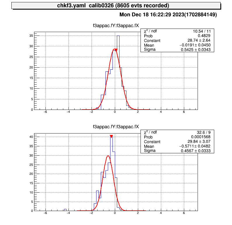
When you complete the setting except for linecalib parameters, let’s start calibration!
We prepared two useful macros to calibrate dl-PPAC.
First, we have to prepare the data with masks on the PPAC like following picture. This mask has holes at 12.5 mm intervals.

The position of the alpha line through the central hole can be calculated and the offset adjusted to achieve that position. The geometry inside the PPAC is as follows. I think all PPAC geometries used by CRIB are the same.
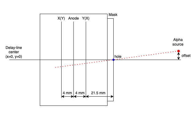
The parameters required to calculate the coordinates of the position are as follows.
Using these parameters, the macro/PPACLineCalibration.C calculate the theoretical position and how much the parameters should be moved.
Let’s calibrate PPACa as an example.
When we set the parameter like this files, the XY figure can be obtained.
Type: art::TPPACParameter
Contents:
  # #2 PPAC
  f3appac:
    ns2mm:
      - 1.256
      - 1.256
    delayoffset:
      - 0.29
      - 0.18
    linecalib:
      - 0.0
      - 0.0
    exchange: 0
    reflectx: 1
    geometry:
      - 0.0
      - 0.0
      - -677.0 # user defined
    TXSumLimit:
      - -800.0
      - 2000.0
    TYSumLimit:
      - -800.0
      - 2000.0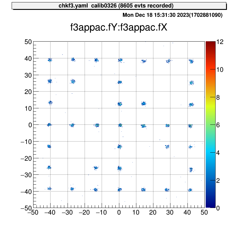
Then we can run the macro.
> acd
> vi macro/run_PPACLineCalibraion.C
# please set the parameters.
# instruction is written in this file

> a
artemis [0] add steering/hoge.yaml NAME=hoge NUM=0000
artemis [1] res
artemis [2] .x macro/run_PPACLineCalibration.C
# -- snip --

===================================================
center position (cal)  : (-0, -0.51413)
center position (data) : (0.890109, -0.274066)
difference             : (0.890109, 0.240065)
move parameters        : (-1.41737, 0.382269)
===================================================
And please input this value to the dlppac.yaml.
Type: art::TPPACParameter
Contents:
  # #2 PPAC
  f3appac:
    ns2mm:
      - 1.256
      - 1.256
    delayoffset:
      - 0.29
      - 0.18
    linecalib:
      - -1.417
      - 0.382
    exchange: 0
    reflectx: 1
    geometry:
      - 0.0
      - 0.0
      - -677.0 # user defined
    TXSumLimit:
      - -800.0
      - 2000.0
    TYSumLimit:
      - -800.0
      - 2000.0
Then you can complete the line calibration of the PPAC.
> a
artemis [0] add steering/hoge.yaml NAME=hoge NUM=0000
artemis [1] res
artemis [2] .x macro/run_PPACLineCalibration.C
# -- snip --

===================================================
center position (cal)  : (-0, -0.51413)
center position (data) : (-0.0191028, -0.571067)
difference             : (-0.0191028, -0.0569366) # <= almost zero!
move parameters        : (0.0304184, -0.0906633)
===================================================
Because of the accuracy of the fitting, it does not make much sense to move the parameters any further.
The PPAC is then ready to be used by measuring how much offset the beamline axis has with respect to the delay-line axis at the position where the PPAC is actually placed, and putting this into the geometry parameters.
H. Kumagai et al., Nucl. Inst. and Meth. A 470, 562 (2001) ↩︎
updating…
This is the CRIB alpha source information. (unit: MeV)
| ID | alpha-2 | alpha-3 |
|---|---|---|
| 4.780 | 3.148 | |
| 5.480 | 5.462 | |
| 5.795 | 5.771 |
SSD calibration files need to be set at prm/ssd/ directory.
The directory structure is like this:
$ tree -L 2 prm/ssd
prm/ssd
├── ch2MeV.dat # test file
├── ch2ns.dat # test file
├── f2ch2MeV.dat
├── f2ch2MeV_raw.dat
├── f2ch2ns.dat
├── tel1
│   ├── ch2MeV_dEX.dat
│   ├── ch2MeV_dEX_raw.dat
│   ├── ch2MeV_dEY.dat
│   ├── ch2MeV_dEY_raw.dat
│   ├── ch2MeV_E.dat
│   ├── ch2MeV_E_raw.dat
│   ├── ch2ns_dEX.dat
│   ├── ch2ns_dEY.dat
│   ├── ch2ns_E.dat
│   └── tel_conf.yaml # telescope configuration, explain later

-- snip --
The prm/ssd/ch2MeV.dat and prm/ssd/ch2ns.dat are used for test, so in the beam time measurement, actually this files are not necessory.
And prm/ssd/f2* files are used for F2SSD calibration, and files in prm/ssd/tel1/ directory are used for SSDs of a telescope.
The ch2ns.dat depends on TDC setting, so basically we don’t have to care so muc
(Usually the setting (the value) is same with previous experiment.), so we have to prepare the ch2MeV.dat files!
The file name need to be set like this example. The loaded parameter file name is defined SSD steering file, and we don’t want to change the SSD steering files so much, so please use such file names.
The “ch2MeV.dat” file format is like this:
# offset gain
1.7009  0.0173
0.0 1.0 # if there are some SSDs or strip SSD, you can add the line.We prepared useful macros to calibrate many SSDs. Please check these for more information.
It is sufficient to use the AlphaCalibration.C, but it is recommended to use the run_AlphaCalibration.C to keep a record of what arguments were used to calibrate.
After you prepared alpha calibration data and steering file (for example steering/calibration.yaml) to show raw data, you can use this macro.
$ acd
$ vi macro/run_AlphaCalibration.C
# please set the parameters.
# instraction is written in this file

$ a
artemis [0] add steering/hoge.yaml NAME=hoge NUM=0000
artemis [1] res
artemis [2] .x macro/run_AlphaCalibration.C
Then the parameter file that defined at the “run_AlphaCalibration.C” and calibration figures will be created automatically.
These are example of the figures;

$ a
artemis [0] add steering/hoge.yaml NAME=hoge NUM=0000
artemis [1] res
artemis [2] fcd 0
artemis [3] zo
artemis [4] tree->Draw("...") # draw calibrated data
artemis [5] gStyle->SetOptStat(0)
artemis [6] sa
updating…
updating…
Analysis files for each experiment are managed using git.
This is so that they can be quickly restored if they are all lost for some reason.
Git is a bit complicated and you can commit freely if you are knowledgeable, but if you are unfamiliar with it, you don’t have to worry too much.
The main use is that if someone creates a useful file, it will be reflected for each user as well.
Here is a brief description of how to use it.
In the CRIB analysis PC, we used local repository. The files related the repository is stored here.
> cd ~
> tree -L 1 repos/exp
repos/exp
├── he6p2024.git
├── he6p.git
└── o14a.git

# 2023/12/18 current statusNote that if you delete the files in this directory, you will lose all backups.
I will describe the most commonly used commands and how to resolve conflicts.
This section explain the example of the online analysis in the CRIB experiment.
From here, we would like to explain in detail how to analyze the actual experiment. We assume that you have already prepared your the analysis environment. It is okay either your own directory or the default directory (see CRIB configuration). If you are not ready yet, please see here.
So let’s start to check the data.
At the F1 focal plane, there is (charge-divition) PPAC.
The steering file to analyze f1 data is chkf1.yaml.
We usually use “chk” (check) as a prefix of the steering files to analyze from raw binaly data.
$ artlogin (username)
$ a
artemis [0] add steering/chkf1.yaml NAME=hoge NUM=0000
artemis [1] res
The important data is “X position” at the F1PPAC. The histogram can be check by following step:
artemis [2] sus
artemis [3] ls

 artemis
>   0 art::TTreeProjGroup f1check         f1_check
    1 art::TAnalysisInfo analysisInfo

artemis [4] cd 0
artemis [5] ls

 f1check
>   0 art::TH1FTreeProj f1ppac_X        f1ppac X
    1 art::TH1FTreeProj f1ppac_Y        f1ppac Y
    2 art::TH1FTreeProj f1ppac_X1raw    f1ppac X1raw
    3 art::TH1FTreeProj f1ppac_X2raw    f1ppac X2raw
    4 art::TH1FTreeProj f1ppac_Y1raw    f1ppac Y1raw
    5 art::TH1FTreeProj f1ppac_Y2raw    f1ppac Y2raw
    6 art::TH2FTreeProj f1ppac_x_y      f1ppac X vs Y
    7 art::TH2FTreeProj f1ppac_x_rf     f1ppac X vs RF
    8 art::TH2FTreeProj f1ppac_x1_x2    f1ppac x1 vs x2
    9 art::TH2FTreeProj f1ppac_y1_y2    f1ppac y1 vs y2
Many histograms are defined, but in practice it’s enough to check the first X position. Sometimes we check other raw data histograms to see if the behavior of F1PPAC is correct or not.
artemis [6] ht 0Usually a gaussian fit is performed to get center the position.
artemis [7] xfFor the commane “xf” (xfitg), please check here.
When you think the signals from F1PPAC is okay, but position seems wrong (the X position is different from the setting of F1 slit), pleace modify the parameter files.
It is actually charge-divition PPAC, but the structure of parameter file is the same with dl-PPAC, so please also check PPAC preparation.
The basic usage is the same.
We use this steering file to check F2 data.
$ artlogin (username)
$ a
artemis [0] add steering/chkf2.yaml NAME=hoge NUM=0000
artemis [1] res
artemis [2] sus
artemis [3] ls

 artemis
>   0 art::TTreeProjGroup f2check         f2_check
    1 art::TAnalysisInfo analysisInfo
artemis [4] cd 0
artemis [5] ls
f2check
> 0 art::TH1FTreeProj f2PPAC X f2ppac x
1 art::TH1FTreeProj f2PPAC Y f2ppac y
2 art::TH1FTreeProj f2SSD raw f2ssd raw
3 art::TH1FTreeProj f2SSD raw (low) f2ssd raw (low)
4 art::TH1FTreeProj f2SSD cal f2ssd cal
5 art::TH2FTreeProj f2PPAC X vs Y f2ppac X vs Y
6 art::TH2FTreeProj F2PPAC X vs RF0 f2ppac X vs rf0
7 art::TH2FTreeProj F2PPAC Y vs RF0 f2ppac Y vs rf0
8 art::TH2FTreeProj RF0 vs F2SSD raw rf0 vs f2ssd raw
9 art::TH2FTreeProj RF0 vs F2SSD cal rf0 vs f2ssd cal
10 art::TH2FTreeProj RF1 vs F2SSD cal rf1 vs f2ssd cal
11 art::TH2FTreeProj F2PPAC X vs F2SSD raw f2ppac x vs f2ssd raw
12 art::TH2FTreeProj F2PPAC X vs F2SSD cal f2ppac x vs f2ssd cal
13 art::TH2FTreeProj F2PPAC Y vs F2SSD cal f2ppac y vs f2ssd cal
14 art::TH1FTreeProj RF0 rf0As you know, you can check the histograms
# for 1D histograms
artemis [*] ht [id]
artemis [*] hn # histogram next
artemis [*] hb # histogram before (back?)
# for 2D histograms
artemis [*] ht [id] colz # colz is option
artemis [*] hn colz
artemis [*] hb colz
If you want to save,
artemis [*] sa
artemis [*] priupdating…
updating…
In the CRIB experiment, we often use a “telescope” consisting of DSSSD (Double-Sided SSD) and SSD (Single-Pad SSD).
The combination of these multiple Si detectors as a dE-E detector is called a telescope.
To analyze the data as telescope data rather than individual detectors, I created a data class called TTelescopeData. This section describes its data structure and usage.
Please assume that one of the name of TTelescopeData object is “tel1”
# after some process
artemis [*] br tel1

 art::TTelescopeData

 Data Members

                 TVector3   fPos                   detected position (X, Y, Z)
                      int   fXID                   X strip number
                      int   fYID                   Y strip number
                      int   fNE                    number of all SSDs
                   double   fdE                    energy at first layor
                   double   fdEX                   X side energy (=~ fdEY)
                   double   fdEY                   Y side energy (=~ fdEX)
                   double   fE                     added energy at thick SSDs
                   double   fEtotal                all energy deposit in the telescope
                   double   fTiming                timing information at the first layor (X side)
                   double   fYTiming               for case that X side have trouble (Y side)
                   double   fTheta_L               reaction angle in LAB system
           vector<double>   fEnergyArray           energy array for each SSD
           vector<double>   fTimingArray           timing array for each SSD
                ESortType   kID
                ESortType   kTiming
               ESortOrder   kASC
               ESortOrder   kDESC

# snip for Method as for now
These are the all data members of the “TTelescopeData”. The most commonly used variables are “fXID”, “fYID”, “fdE” and “fE”. Other variables are accessed by using methods (explain later). The meaning of these variables are written the upper code block.
We use them like,
artemis [*] tree->Draw("tel1.fYID:tel1.fXID>>strip(16,-0.5,15.5, 16,-0.5,15.5)","","colz")
artemis [*] tree->Draw("tel1.fdE:tel1.fE","","")
or we can use in histogram definition file of course.
The following are the methods of the TTelescopeData object:
# after some process
artemis [*] br tel1

# snip for Data Members

 Methods

          TTelescopeData&   operator=
                 TVector3   GetPosition
                 Double_t   X
                 Double_t   Y
                 Double_t   Z
                     void   SetPosition
                     void   SetPosition
                    Int_t   GetN
                     void   SetN
                    Int_t   GetXID
                     void   SetXID
                    Int_t   GetYID
                     void   SetYID
                 Double_t   GetdE
                     void   SetdE
                 Double_t   GetdEX
                     void   SetdEX
                 Double_t   GetdEY
                     void   SetdEY
                 Double_t   GetE
                     void   SetE
                 Double_t   GetEtotal
                     void   SetEtotal
                 Double_t   GetTelTiming
                     void   SetTelTiming
                 Double_t   GetTelYTiming
                     void   SetTelYTiming
                 Double_t   GetTheta_L
                     void   SetTheta_L
                 Double_t   A
              DoubleVec_t   GetEnergyArray
                 Double_t   GetEnergyArray
                     void   PushEnergyArray
              DoubleVec_t   GetTimingArray
                 Double_t   GetTimingArray
                     void   PushTimingArray
                 Double_t   E
                 Double_t   T
                     void   Copy
                     void   Clear
                   Bool_t   CheckTObjectHashConsistency

 See also

     art::TDataObject       base class for data object
The most commonly used methods are “X()”, “Y()”, “Z()”, “E()”, “T()” and “A()”. There are also longer name methods, but it is troublesome to write long methods, so I prepared short name methods. The longer name methods are mainly used in the source processor to make it more readable.
X(): return fPos.X(), detected X positionY(): return fPos.Y(), detected Y positionZ(): return fPos.Z(), detected Z positionE(): return fEtotal, total energy deposit in the telescopeE(id: int): return fEnergyArray[id], energy deposit of each Si layer, id=0 means dE, id=1 means second layerT(): return fTiming, detected timing at first layerT(id: int): return fTimingArray[id], timing at the “id” th Si detectorA(): return fTheta_L, the angle of the event, deg unitWe use them like:
artemis [*] tree->Draw("tel1.Y():tel1.X()","","colz")
artemis [*] tree->Draw("tel1.E(0):tel1.E()","","colz")
artemis [*] tree->Draw("tel1.E():tel1.A()","","colz")In the physics run (production run or physics measurement), we check all the detector data like tracking detector (PPAC, MWDC), TOF (RF) and Telescope data. In order to analyse them, we prepared steering/chkf3.yaml steering file. This file includes all the information of F3 analysis.
$ artlogin (username)
$ a
artemis [0] add steering/chkf3.yaml NAME=hoge NUM=0000
artemis [1] res
artemis [2] sus
artemis [3] ls

 artemis
>   0 art::TTreeProjGroup f3check         f3check
    1 art::TAnalysisInfo analysisInfo
    2 art::TTreeProjGroup mwdca           mwdca
    3 art::TTreeProjGroup mwdcb           mwdcb
    4 art::TTreeProjGroup tel1            tel1
    5 art::TTreeProjGroup tel2            tel2
    6 art::TTreeProjGroup tel3            tel3
    7 art::TTreeProjGroup tel4            tel4
    8 art::TTreeProjGroup tel5            tel5
    9 art::TTreeProjGroup tel6            tel6
   10 art::TTreeProjGroup MUX             MUX
   11 TDirectory MWDCCalibHists  MWDC calibration

# this is the situation at 2024/01/22
There are many histogram definition, and you can freely update the histogram files.
Because this file contains most of the knowledge about the steering file, so you can test your own histogram or something based on this file.
$ cd steering
$ cp chkf3.yaml chkYourOwnName.yaml
$ vi (emacs) chkYourOwnName.yaml
# change or test something

$ acd
$ a
artemis [0] add steering/chkYourOwnName.yaml NAME=hoge NUM=0000
artemis [1] res
artmeis [2] sus

# some analysisIt is very important to select events for online analysis as well. There are several options to do so, and I will cover all of them. If you know other useful way, please let me know.
For clearer understanding, we will use this figure, and we call this as default figure:

We explained in the Histograms page, but again we describe about histogram definition focus on the cut part.
The default figure defined like this:
anchor:
  - &f2ppacx ["f2ppac.fX",200,-50.,50.]
  - &f2ppacy ["f2ppac.fY",200,-50.,50.]
alias:
group:
  - name: f2check
    title: f2_check
    contents:
      - name: f2PPAC X vs Y
        title: f2ppac X vs Y
        x: *f2ppacx
        y: *f2ppacy
For example, let’s add the gate to select only “-10.0 < X < 10.0”. We can use alias node to define that.
anchor:
  - &f2ppacx ["f2ppac.fX",200,-50.,50.]
  - &f2ppacy ["f2ppac.fY",200,-50.,50.]
alias:
  centerx: abs(f2ppac.fX) < 10.0;
group:
  - name: f2check
    title: f2_check
    contents:
      - name: f2PPAC X vs Y{centerx}
        title: f2ppac X vs Y{centerx}
        x: *f2ppacx
        y: *f2ppacy
        cut: centerx
Then the following histogram is created.

Also, multiple conditions can be specified at the same time.
anchor:
  - &f2ppacx ["f2ppac.fX",200,-50.,50.]
  - &f2ppacy ["f2ppac.fY",200,-50.,50.]
alias:
  centerx: abs(f2ppac.fX) < 10.0;
  centery: abs(f2ppac.fY) < 10.0;
group:
  - name: f2check
    title: f2_check
    contents:
      - name: f2PPAC X vs Y{centerx && centery}
        title: f2ppac X vs Y{centerx && centery}
        x: *f2ppacx
        y: *f2ppacy
        cut: centerx && centery
We can also use TCutG object to select the event.
As in new commands page, let’s assume we create this TCutG ROOT file by tcutg command.
And the ROOT file and TCutG object name is f2star.

If you want to use this object to select event, just add this line is fine, as long as you use userlogon.C.
anchor:
  - &f2ppacx ["f2ppac.fX",200,-50.,50.]
  - &f2ppacy ["f2ppac.fY",200,-50.,50.]
alias:
group:
  - name: f2check
    title: f2_check
    contents:
      - name: f2PPAC X vs Y{f2star}
        title: f2ppac X vs Y{f2star}
        x: *f2ppacx
        y: *f2ppacy
        cut: f2star
Of course we can use in “tree->Draw()” because this TCutG objects are automatically loaded. The following sentence generate the same figure.
artemis [] fcd 0
artemis [] zo
artemis [] tree->Draw("f2ppac.fY:f2ppac.fX>>(200,-50.,50., 200,-50.,50.)","f2star","colz")The method used until now was to process just histograms and analyze them for all events in the event loop. If you know which events you don’t want, there are processors that allow you to skip the event loop under certain conditions. This may speed up the event loop.
For example. when we want to analyze only beam single event (it means the events are not coincident with SSD, and let’s suppose that condition is given by single.fID==0), let’s prepare the steering file.
Processor:
  - name: proc_gateinit
    type: art::TGateArrayInitializer
    parameter:
      OutputTransparency: 1

  - name: proc_gate
    type: art::TTreeFormulaGateProcessor
    parameter:
      Definitions:
        - "beam_single; single.fID==0"
      OutputTransparency: 1
      Verbose: 1

  - name: beam_single_gate
    type: art::TGateStopProcessor
    parameter:
      GateName: beam_single
      OutputTransparency: 1
      StopIf: 0
      Verbose: 1
To use TGateStopProcessor, we need to initialize the “gate” array object, so the first art::TGateArrayInitializer is needed.
In the second processor, art::TTreeFormulaGateProcessor, we define the gate condition.
Then the art::TGateStopProcessor judges the event is skipped or not.
In the case of StopIf: 0, artemis ignore the event that the condition become false.
In other words, StopIf: 0 means artemis will analyze the event only when the condition is true.
Then, including this yaml file to the main steering file, you can check only the selected events.
Anchor:
  - &input ridf/@NAME@@NUM@.ridf
  - &output output/@NAME@/@NUM@/hoge@NAME@@NUM@.root
  - &histout output/@NAME@/@NUM@/hoge@NAME@@NUM@.hist.root

Processor:
  - name: timer
    type: art::TTimerProcessor

  - name: ridf
    type: art::TRIDFEventStore
    parameter:
      OutputTransparency: 1
      InputFiles:
        - *input
      SHMID: 0

  - name: mapper
    type: art::TMappingProcessor
    parameter:
      OutputTransparency: 1

# include some other steering files

  - include: gate/coin.yaml

  - name: outputtree
    type: art::TOutputTreeProcessor
    parameter:
      FileName:
- *outputWe didn’t check if we can use the TCutG object in this process…
Artemis produces mainly TArtTree and the branches are TClonesArray(art::hoge).
It means that all objects rely on the artemis library, and we cannot open and check the data by using normal ROOT.
Also, sometimes it is necessary top check the raw data obtained by ADC and TDC as it is. Of course, the real raw data is binary and therefore difficult to read, so we will check the raw data after the decoders.
Related processors;
We already prepared conf/map files, but in this case, we need to prepare conf/seg files.
There are two files.
This is an example, so please change it according to the experimental conditions.
#modulename:
#  id: module id (it is module-specific)
#  ch: channel number
#  values:
#    - name1: [Nbin: int, min: double, max: double] it is for 2D histogram (these values vs. ch)
#    - name2: [Nbin: int, min: double, max: double] <= somehow two line needed...?

MADC32:
  id: 32
  ch: 32
  values:
    - adc: [4000, 0., 4000.]
    - tdc: [4000, 0., 4000.] # no use, but seems it needed...

V1190A:
  id: 24
  ch: 128
  values:
    - tdcL: [300, -5000., 300000.]
    - tdcT: [300, -5000., 300000.]
The module id list is here.
#segment_name:
# segid: [[dev], [fp], [det]] <= same as a map file
# type: V7XX <= defined type in modulelist.yaml
# modules:
#   - id: geo1
#   - id: geo2

V1190:
  segid: [12, 0, 7]
  type: V1190A
  modules:
    - id: 0
    - id: 1

MADC:
  segid: [12, 1, 6]
  type: MADC32
  modules:
    - id: 0
    - id: 1
- id: 2Based on these two conf file, the steering/chkseg.yaml file produce rawdata histograms and TTree object.
We can use steering/chkseg.yaml without any change I think.
This is an example from one CRIB experiment.
$ a
artemis [0] add steering/chkseg.yaml NAME=hoge NUM=0000
artemis [1] res
artemis [2] sus
artemis [3] ls

 artemis
>   0 TDirectory SegmentHistogram art::TSegmentCheckProcessor

artemis [4] cd 0
artemis [5] ls

 SegmentHistogram
>   0 TDirectory E7_V1190        E7_V1190
    1 TDirectory J1_V785         J1_V785
    2 TDirectory J1_MADC         J1_MADC
    3 TDirectory J1_V1190        J1_V1190

artemis [6] cd 0
artemis [7] ls


 E7_V1190
>   0 TH2F E7_V1190_0_tdcL E7_V1190_0_tdcL
    1 TH2F E7_V1190_0_tdcT E7_V1190_0_tdcT
    2 TH2F E7_V1190_1_tdcL E7_V1190_1_tdcL
    3 TH2F E7_V1190_1_tdcT E7_V1190_1_tdcT

# we can check these histograms by ht command

artemis [8] fcd 0
artemis [9] br
E7_V1190_0           vector<vector<int> >
E7_V1190_1           vector<vector<int> >
J1_V785_0            vector<int>
J1_V785_1            vector<int>
J1_V785_2            vector<int>
J1_MADC_3            vector<int>
J1_MADC_4            vector<int>
J1_MADC_5            vector<int>
J1_V1190_0 vector<vector<int> >If the module ID = 24 or 25, it is multihit TDC, so the branch become 2D vector. When you want to use std::vector method, you can use by “@” like
artemis [*] tree->Draw("J1_V785_0@.size()")Of course we can open this output ROOT file from normal ROOT.
This section explain the example of the offline analysis (some useful processors).
A brief example of an analysis flow using artemis_crib is given below. This is just the method recommended by okawak, so you can proceed with the analysis as you like.
I hope this page will give you some ideas.
The acquired data contains a lot of noise and other data that is not absolutely necessary for analysis,
and if you use artemis to do an event loop for all events, it will take a long time.
Therefore, a root file should only be created for a specific RUN (data file) to save time.
(It is tempting to look at the data using with a lot of statistics,
but we believe that this is done by online-analysis and concentrate on reducing useless data.)
$ artlogin (user)
$ a

artemis [] a steering/hoge.yaml NAME=run NUM=0000
artemis [] .q
As you want to look at a variety of data I think, it is convenient to create a canvas each time with ‘tree->Draw()’, instead of defining a histogram. Not defining a histogram also has the advantage that the event loop is faster.
Once the root file has been created, it can be read directly from that file, eliminating the waiting time.
$ a output/created_rootfile_path.root

artemis [] tree->Draw("hoge")
It is good idea to make a “.C” macro file to record and reproduce the analysis process.
Here are some points I think would be good to check:
If there are problems during the experiment, there may be many other things to check.
It is possible that some parameter is different for each RUN. There are many possibilities, for example, a trouble may have occurred and the conditions of the detector have changed. In such cases, it is necessary to take action, for example, to prepare several calibration parameters.
While some of these changes in parameters can be predicted in advance, unforeseen changes can also occur.
These are the problems I have encountered, but others with different tendencies may exist.
If you can anticipate it, it is good to have a plan for dealing with it at this point and move on to the next step. However, there is no need to waste time here as it can be noticed after merging the overall measurements in the following step.
This section explain the example of the Monte Carlo simulation by using artemis.
It is very useful to use Monte Carlo (MC) simulation to obtain various calculated values. From this section, we will show the simple example how to perform MC simulation using artemis.
First, we will set the generator of the beam that will bombard on the target. We have two kinds of generator:
After you get beam information from a measurement, second option might be useful.
This is an example of a steering file.
Processor:
  - name: random_eventstore
    type: art::TRandomNumberEventStore
    parameter:
      OutputTransparency: 1
      MaxLoop: *loopnum

  - name: beam_generator
    type: art::TRandomBeamGenerator
    parameter:
      OutputCollection: *beam_name
      OutputTrackCollection: *track_name
      #beam particle information
      MassNum: *beam_A
      AtomicNum: *beam_Z
      ChargeNum: *beam_Z
      IniEnergy: *beam_E
      #beam tracking information
      Xsigma: 1.0 # mm
      Ysigma: 1.0 # mm
      Asigma: 1.0 # deg
      Bsigma: 1.0 # deg
      Esigma: *beam_Esigma
This produces two branch, “beam” and “track”.
Actually “track” information is contained in “beam” branch.
Here is the detail of the type of “beam”.
artemis [] classinfo art::TParticleInfo

 art::TParticleInfo

 Data Members

                      int   fMassNumber
                      int   fAtomicNumber
                      int   fCharge
                   double   fEnergy                kinetic energy in LAB system
                   double   fCurrentZ              current Z position
                   double   fTime                  Duration time (ns)
                   TTrack   fTrack                 tracking information in LAB system
           TLorentzVector   fVec                   lorentz vector (px, py, pz, E) of this particle
                   double   fTheta_cm              theta angle (deg) in CM system
                   double   fPhi_cm                phi angle (deg) in CM system

-- snip --
fCurrentZ is the current Z position and at the beam generation, this value will be set as 0 after this processor.
For example, the beam angle distribution will be like this.
The tracking information obtained from the experiment can also be used to generate the beam. In the current version, the position and angle of the beam are read from a ROOT file and the energy is given randomly.
This is an example of a steering file.
Processor:

  - name: periodic_tree
    type: art::TTreePeriodicEventStore
    parameter:
      OutputTransparency: 1
      FileName: *input
      TreeName: tree
      MaxEventNum: *loopnum

  - name: proc_copy_processor
    type: art::TBranchCopyProcessor
    parameter:
      InputCollection: f3ppac # need to inherit from TTrack
      OutputCollection: *track_name

  - name: beam_generator
    type: art::TTreeBeamGenerator
    parameter:
      InputCollection: *track_name
      OutputCollection: *beam_name
      # beam particle information
      MassNum: *beam_A
      AtomicNum: *beam_Z
      ChargeNum: *beam_Z
      IniEnergy: *beam_E
      Esigma: *beam_Esigma
It reads an object named “f3ppac”, which inherits from TTrack, from a TTree named “tree” in a file named “*input”,
and creates an object of the same type as before named TParticleInfo.
make a reaction considering phase space.
  - name: reaction_proc
    type: art::TNBodyReactionProcessor
    parameter:
      InputCollection: *beam_name
      OutputCollection: products # size is DecayParticleNum
      OutputReactionCollection: reaction
      # beam information (for initialize TSrim)
      BeamNucleus: [*beam_Z, *beam_A] # (Z, A)
      BeamEnergy: *beam_E
      # target information
      TargetIsGas: true # false-> solid, true-> gas target
      TargetName: he # from TSrim energy loss
      TargetMassNum: 4 # hit ion
      TargetAtomicNum: 2 # hit ion
      TargetThickness: 1000 # mm (for gas target, allow up to this value)
      TargetPressure: 250 # Torr (used for gas target)
      # reaction particles information
      DecayParticleNum: 2
      ReactionMassNum: [29, 1] # will be [id=0, id=1]
      ReactionAtomicNum: [15, 1]
      ExciteLevel: [0.0, 0.0] # MeV
      # cross section file, if not, it use constant cross section for energy
      # require: "energy cross-section" format, deliminator should be a space ' '
      CrossSectionPath: path/to/cs/file
      CrossSectionType: 0 # 0-> LAB, kinematics is different, 1-> LAB, kinematics is same, 2-> CM
NOTE
TargetName that registered this library# comment
# energy cross_section
0.0 0.0
0.1 1.0 # comment
# 0.2, 2.0 camma is not allowed...products is size two array, like products[0] -> id=0 particlereaction contain reaction information, like Ecm, Thetacmartemis [] classinfo art::TReactionInfo
art::TReactionInfo
Data Members
double fEnergy / Ecm of the reaction
double fTheta / Thetacm of the reaction
double fX / reaction position at LAB system, x
double fY / reaction position at LAB system, y
double fZ / reaction position at LAB system, z
double fExEnergy / excited energy of residual nucleus
ESortType kID
ESortType kTiming
ESortOrder kASC
ESortOrder kDESC We will show an example of a simulation performed for a gas target case like the steering file above. (of course we can use it also for solid target case!)
Details of the reactions that took place are shown in these figures.
The reaction cross section files are appropriately specified.
This figure is the reaction energy at CM system.
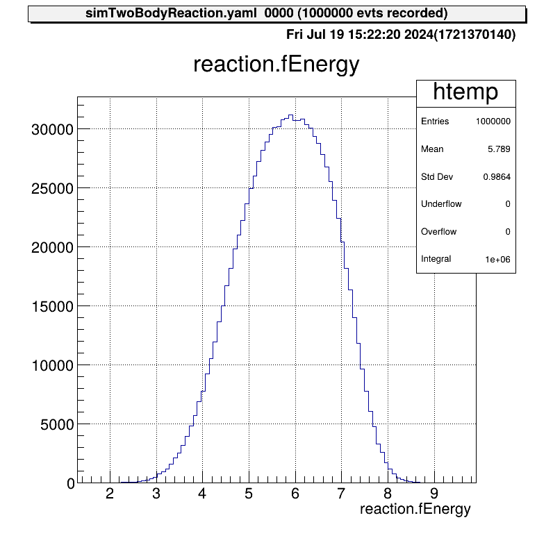
This distribution was created from a file of reaction cross section. The effect of beam energy spread is included, so the edge of the peak is not sharp.
According to this energy distribution, the distribution of the positions of the reactions is as follows.
The angular distribution at CM system of reactions is assumed to be uniform. This figure shows the direction of one particle that is produced from this reaction.
Also the relationship between the kinematics of the reactions will be like this.
Configure detector geometry to judge if the reaction particle hit the detector or not.
material:
  - name: Vaccum # id=0
    atomic_mass: 0.0
    atomic_num: 0.0
    density: 0.0 # g/cm3

  - name: Si # id=1
    atomic_mass: 28.084
    atomic_num: 14.0
    density: 2.321

# Note: beam axis -> z, upper direction -> y
conposition:
  detector:
    - name: tel1
      strip: [16, 16]
      center_rotation: [0., 0., 322.0] # mm
      offset: [0., 0., 0.]
      distance: 244.0
      angle: -4.0 # deg
      thickness: [0.02, 0.301, 1.494, 1.486]
      pedestal: [0., 0., 0., 0.] # MeV, below this energy, assume 0 MeV
      material: [Si]

    - name: tel2
      strip: [16, 16]
      center_rotation: [0., 0., 322.0]
      offset: [0., 0., 0.]
      distance: 154.5
      angle: 27.0
      thickness: [0.02, 0.300, 1.494, 1.485]
      pedestal: [0., 0., 0., 0.] # MeV, below this energy, assume 0 MeV
      material: [Si]

volume:
  top: # detector world
    name: TOP
    type: box # now only box is available
    material: 0
    size: [400.0, 200.0, 1288.0] # mm

  detector:
    - name: tel1
      type: box
      material: 1
      size: [50.0, 50.0, 1.0] # mm

    - name: tel2
      type: box
      material: 1
      size: [50.0, 50.0, 1.0] # mm
The geometry information is used only for the judgement, so any material is actually okay.
The material node is used to define TGeoMaterial and TGeoMedium classes.
From name to density node are used to make a instance of this object.
This values are not used in the current processors.
The next conposition node define the detector configuration.
General telescopes of the CRIB experiment consist of DSSSD and SSD (single-pad),
and the node below defines the SSD of the telescope.
SRIMlib calculation. This node is defined as a array for each layer, but if it is one, the same material is applied. For example, in example.yaml, [Si] means [Si, Si, Si, Si]. (You need to prepare SRIMlib setting beforehand!)As for the node is center_rotation, offset, distance and angle, please see this figure.

Please note that the center_rotation and offset are defined in (x, y, z) coordinate, and distance and angle are scalar value.
The unit of length is mm, angle is deg.
The sign of the angle is defined as positive at this figure (right-hand system). And generally, we set z=0 at target position. (For the gas target, we set 0 at window position.)
The last part volume node, the shape of the detector will be defined by using TGeoVolume class.
The TGeoVolume needs name, type, material and size.
For the type, I only prepared “box”. (It means the code use only vol->MakeBox method.)
The first top node must be set because it defined “detector world”.
Generally, the material is okay to set vaccum.
And the material is defined in the material node, and the id (the order) can be used.
So the format is like material: 0.
And the size is generally set to the size of the scattering chamber, but for the safety, it is okay to set larger number.
Also the unit is mm and format is (x, y, z).
Next, at the volume/detector node, we can define the detector size.
NOTE: the volume/detector/name should be the same with conposition/detector/name node.
Then, let’s check if the parameter file can be correctly used.
Anchor:

Processor:
- name: detector_initialize
  type: art::TUserGeoInitializer
  parameter:
    FileName: prm/geo/example.yaml
    Visible: true
    OutputTransparency: 1
This steering file doesn’t use event loop. Just we want to check the parameter file works well or not.
Then let’s see in the artemis!
$ acd
$ a

-- snip --

artemis [0] add steering/geo_example.yaml

-- snip --

artemis [1] ls

 artemis
>   0 TGeoVolume TOP             Top volume

artemis [2]
The detector geometry object is successfully generated! In order to check the object, please use draw command for example. (It is defined only in CRIB artemis, to draw not only histogram object. This is under development.)
Or you can get the object with some methods and obj->Draw() will work.
artemis [2] draw 0
The red box is the TOP, and the black boxes are detectors. If the detector is placed where you expect it to be, the parameters have been successfully set!
Using the defined reactions (TNBodyReactionProcessor) and geometry (TUserGeoInitialiser) so far, it is possible to determine whether the particles enter the detector after the reaction and to simulate the parameters obtained.
  - name: detector_proc
    type: art::TDetectParticleProcessor
    parameter:
      InputCollection: products
      InputTrackCollection: track
      OutputCollection: detects
      # target information (use if gas target)
      TargetIsGas: *target_is_gas # true -> gas target
      TargetName: *target_name
      TargetPressure: *target_pressure # Torr (used for gas target)
      EnergyResolution: [0.0] # x 100 = %, det id = 0, 1, ..
products is an array object of produced ions [id=0 ion, id=1 ion…]detects is an array object of detected ions [id=0 ion, id=1 ion…]We will show an example of a simulation performed for a gas target case, and resolution = 0.0.
First, this is a figure of the detected position of light particle. We defined five telescopes in this example, and we can clearly see the position of the detectors. If we focus on heavy particle, we cannot see the position distribution because all ions are stopped in the gas target.

As an example, we will show you figures of a telescope with the largest angle. Here is dE-E plots.

The relationship between energy and timing is like this.

Also, here is the angular distribution of the LAB system.

The processor created by okawak allows simple simulations to be performed without creating new sources, if the following conditions are met.
There are only two files that need to be prepared for the simulation.
prm/geo/hoge.yaml -> define detector configuration (example prm/geo/si26a.yaml)
currentsteering/huga.yaml -> define simulation parameters (example steering/simNBodyReaction.yaml)As an application of the above four sections, I would like to explain how to calculate solid angles using Monte Carlo methods!
When you start the event loop in online mode and artemis gets stuck, babian may not have been activated.
There is a shellscript to run the “babian” in cribana PC.
~/bin/run_babian
ps aux | grep babi # check if the "babian" process is working or notchkridf command shows like this:
chkridf hoge.ridf-- snip --
:
Segment Header / blkn=1
hd1 = 0x2100004c
ly=2, cid=4, size=76, efn=120
Segment ID = 12600853 (0x00c04615)
Rev 0 / Dev 12 / FP 1 / Det 6 / Mod 21
2000 0200 4072 0000 406c 0010 405f 0001
4068 0011 406a 0002 4053 0012 4058 0003
4058 0013 4051 0004 4066 0014 404d 0005
4047 0015 4045 0006 4056 0016 405a 0007
404b 0017 4050 0008 406c 0018 404b 0009
4069 0019 4059 000a 4051 001a 404e 000b
405f 001b 4064 000c 4052 001c 4033 000d
4055 001d 4064 000e 4067 001e 4043 000f
4052 001f 1dd2 0401 1dd2 0601
-- snip --If you forgot to “git pull” and you have already modified the files, you will get conflicts. If you think it is okay to forget your modified file, please command like
$ git stashand
$ git pullAnd you want to recover your modified file,
$ git stash popThen you encounter the conficts again, and please select the code you want to keep, and git push again. For the detail, please check here.